In the first article of this series, we outlined the problem: our fictional CEO wants to predict taxi use to ensure taxis are available where and when customers need them. In the second article, we imported our SQL data into Azure and built the model to solve the problem. In this article, we dig into using the output from the model to give the CEO what they need to run the business.
We access our experiments through the Azure Machine Learning Studio, similar to Azure Synapse Analytics’ studio interface. We can observe the running and completed jobs through this interface, including information about the jobs, errors, and the ML engine itself. We can also get statistical output from the models.
Our model exists as a programmatic model, and we test it by firing input variables at it. Based on the input, the model determines what the output should be.
Looking at the Model Details
When we open Azure Machine Learning Studio, it presents us with a list of recent runs. We can determine the status of our run using this screen.

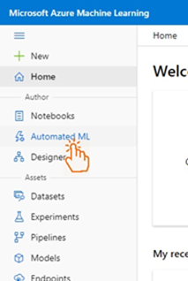
We can select to view only the Automated ML runs by clicking that option in the menu, as the screenshot below demonstrates:
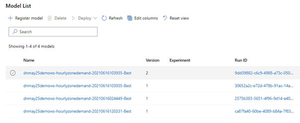
The Models menu item displays the best model, which the machine learning engine flags.
The resultant statistics (metrics) are available for each run.

The interpretability package in the Azure SDK for Python can tell us more about our model by explaining model behavior.
Once it completes its operations, the engine generates specific files as part of its output. These files aid in deploying the consumption model.
Getting the Inputs in and the Outputs Out
There are two methods available for consuming the model: a real-time endpoint or a web service. For our purposes, we use the web service.
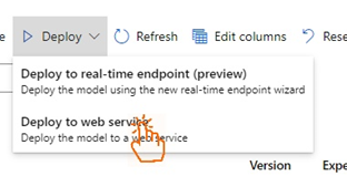
We need to upload a few files to create the web service. We need a Python file to initialize the web service and add the required dependencies.
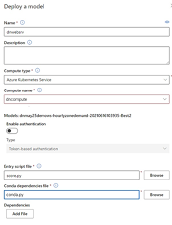
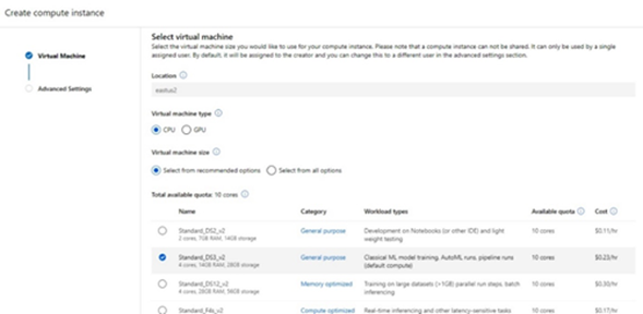
We create a compute instance when deploying our model to be able to execute the model. Other files contain required dependencies, and we can select from a list of configurations for our compute instance.
We need a Python script file called the Entry Script to define the interface for the web service. When we deploy the web service, Azure Machine Loading Studio uploads this and other files. The Python script consists of an init function and a run function.
We can define our input and output data structures within the init function. For example:
import joblib
import json
import numpy as np
import os

from inference_schema.schema_decorators import input_schema, output_schema
from inference_schema.parameter_types.numpy_parameter_type import NumpyParameterType

def init():
    global model
    model_path = 'azureml-models/dnmay25demows-hourlyzonedemand-20210616103935-Best/2/dnmay25demows-hourlyzonedemand-20210616045820_artifact/model.pkl')
    # Deserialize the model file back into a sklearn model.
    model = joblib.load(model_path)

input_sample = np.array([[1068143, 2017, 10, 14, 11, 7]])
output_sample = np.array([4])

@input_schema('data', NumpyParameterType(input_sample))
@output_schema(NumpyParameterType(output_sample))
def run(data):
    try:
        result = model.predict(data)
        # You can return any JSON-serializable object.
        return result.tolist()
    except Exception as e:
        error = str(e)
        return error
When we call the web service passing the input parameters in a JSON structure, we can read our results from a JSON structure in the response.
Now, we need to write a routine to query the web service, using a simple Python script like this:
import requests
import json

ws_uri = '<web service URI>'
key = '<security key or token>'

data = {"data":
        [
            [
                2017,
                1,
                1,
                17,
                1
            ]
        ]
        }
# Convert to JSON
input_data = json.dumps(data)

headers = {'Content-Type': 'application/json'}
headers['Authorization'] = f'Bearer {key}'

ws_response = requests.post(ws_uri, input_data, headers=headers)
print(ws_response.text)
Our model returns a JSON structure containing the most probable solution given the inputs. In our model, simply a single integer.
We can supply several input arrays stacked in the data structure and get an array of individual results.
Since the web service is a standard call, we can use the language of our choice. Microsoft provides several examples of how to consume your model.
Get Our Results Back into SQL
One of the conveniences of working with Azure Synapse Analytics is its ability to integrate. We can create a table in SQL Server and query it in Azure Spark. The reverse is also true.
Our model consists of two separate parts, so we end up with two web service endpoints. We must now make our first call to the "get routes" web service. We pass the data to our web service, and it returns a list of the most likely trips customers will take on that date.
We now split the returned list then build a data structure using the same information plus the trip index. Then, we pass this structure to the "get demand" web service.
The web service returns the expected number of calls for that trip. We write this data to a Python DataFrame then write the DataFrame to a table in our dedicated SQL server. A Python notebook example shows you how to get a DataFrame into your dedicated server, although we will have to adjust the exact code to our specific needs.
In our case, we use a PySpark notebook to call the web services. The notebook saves the results in a table called FcstZoneDemand on our dedicated SQL Server instance. The table structure is as follows:


Once our table populates, we can execute the stored deployment procedure. This procedure compares the expected demand with the expected supply and determines where an under-supply exists. It then determines the best source to balance that shortage. Finally, it writes these results to a deployment table as a proposed deployment schedule.
Analyzing Our Results
Our data sits in Parquet tables and are queried using SQL queries on our Azure serverless database. Our dedicated instance holds the zone distance data to speed up deployment. We did not write the process efficiently, but it works.
The output from the forecasting model sits on our dedicated SQL database in a table called "FcstZoneDemand." Two supplementary tables add to the deployment process: the forecast period under and oversupply details.
When we join these tables on forecast period and zone, the result enables us to view the coming periods. We can see how the deployment balances supply and demand. Using Power BI, we can give the CEO the information they need to make their decisions.
The chart below is from the Synapse Studio SQL script editor, where we can view our data as a chart and download it as an image. This chart shows the expected demand our model generated. We can visualize how the demand changes at a single zone over 24 hours. From this demand, we can see where and when there are too many vehicles and too few vehicles.

In this case, the suggested deployment lined up with the undersupply, so there was enough supply from nearby zones to cater to the demand. If that undersupply is greater than what is available, there will be a wait for a taxi in that zone.
This chart shows the suggested supply as a total. The deployment model draws supply from the closest zones up to the available supply. After that, it looks at the next nearest zone, continuing until the demand is in balance.
Looking at the output, we are happy that the forecast represents reality. The oversupply at the start of the working day suggests this might be a commercial zone. People might take taxis from other zones to drop them off here. At the end of the day, the demand increases as people call for taxis to go back home.
The CEO should be happy with this cost-effective overnight solution.
Next Steps
In the first article of this series, we discussed how to use Azure Synapse Analytics to convert our SQL data into a model to ensure our company’s taxis are available when and where customers need them. In the second article, we imported data from an existing SQL Server. We employed a machine learning model to predict taxi demand and send our vehicles to the locations that need them. Then, in the current article, we explored how to retrieve the machine learning results and view that data.
Although this article explored using Azure Synapse Analytics with SQL data to predict and respond to taxi demand, you can use the same techniques for similar supply-and-demand situations, from services to products. These tools use your existing data to find the insights you need to make efficient business decisions.
To learn more about how Azure Synapse Analytics can help your organization make the most of your data, register to view the Hands-on Training Series for Azure Synapse Analytics. With each session led by an Azure Synapse engineer, this series teaches you to:
- Start your first Synapse workspace
- Build code-free ETL pipelines
- Natively connect to Power BI
- Connect and process streaming data
- Use serverless and dedicated query options
