Introduction
A rectangle in general position in space is seen by a
camera as a quadrilateral. Any point inside the rectangle projects to a point
inside the quadrilateral. This article is about how the mapping of any point
can be found, given the projections of the four corners.
We will establish the necessary equations, to compare
to the well-known bilinear interpolation method and highlight the inaccuracy of
the latter for this purpose.
The Bilinear Transform
Let us discuss the bilinear transform first. A very
simple way to map the original rectangle to the quadrilateral is by linear
interpolation along the sides.
First we perform a linear interpolation along two
opposite sides, using an interpolation parameter  . Then we interpolate between these two interpolated
points, using a second interpolation parameter, . Given the four projected corners , clockwise,
we have:
. Then we interpolate between these two interpolated
points, using a second interpolation parameter, . Given the four projected corners , clockwise,
we have:
and:
or simply:
You can check for yourself a nice property of this
scheme: if you start interpolating on the other pair of sides (03, 12) instead
of (01, 32), you will get exactly the same result.
Note that by this definition, any grid line with or constant
is transformed into a straight line. (But arbitrary lines are transformed into
a curve - a conic curve.)
The Homographic Transform
Establishing the true projection equations will
require some more effort. First, we will establish the general form of the
equations, then the way to compute any unknown parameter they comprise.
From spatial geometry, we know that a rigid object is
moved in space by applying to it a rotation and a translation. A rotation is
described by a 3x3 matrix which is applied to the original coordinates, and the
translation by a 3-vector which is added. In our case, the rectangle lies in a
plane so that one of the input coordinates is identically 0.
Hence the transformation equations:
Then the projection itself is achieved by reducing the
coordinates
in the inverse proportion of the distance:
with being
a constant called the focal length of the camera, that we can absorb in the
constants above.
We obtain a so-called homography:
The nine coefficients can be multiplied by a common
arbitrary factor, and without loss of generality, we can assume , to get:
To determine the 8 unknown coefficients, we use the
coordinates of the projections of the four corners, let ,
corresponding to and , in
clockwise order and replace them in the general expression:
The bad news: this gives us a nonlinear system of 8
equations in 8 unknowns ( to ), something
usually painful to solve.
The good news: the system can be linearized and
simplified to such an extent that the solution becomes straightforward.
First, we translate all by so
that becomes
the origin; we denote the new vertices . This makes the coefficients and vanish
because:
Two unknowns are gone!
Next, we linearize by moving the denominator to the
left-hand side and rearranging the terms:
When we substitute by their values at , and , we get
these six equations:
By introducing , and , we get a
further simplification (this is a little rabbit out of a hat – but it is
optional):
<to id="_x0000_i1044" src="/KB/recipes/674433/image062.png" height="16" width="12" border="0">and we
subtract equations 1 and 5 from 3, and 2 and 6 from 4, yielding (note the new
indexes):
Solving this 2x2 system in and by
Cramer's rule is trivial, and , , , , , immediately
follow.
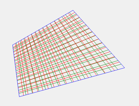
The accompanying demo application will show you the
discrepancies between the bilinear and perspective transforms, which is
particularly noticeable for skewed quadrilaterals. On the opposite, for
parallelograms both transforms become affine and coincide exactly.
When the quadrilateral is not convex, the perspective
transform shows "erratic" behavior. This is because such cases are
not physically achievable.
Background
General understanding of
analytic geometry and perspective transforms is assumed.
Using the Code
The code directly reflects
the equations established in the article and is just meant to illustrate these.
The chosen language is irrelevant.
Drag the quadrilateral
corners with the mouse.
Points of Interest
While working on the
homographic equations, I was amazed to see how easily they can be solved in the
case of a rectangle.
History
This is the first version.

