Introduction
LMS algorithm is one of the most popular adaptive algorithms because of its simplicity. Computing LMS does not require computing of correlation matrix, or even computing of matrix inversions. Indeed, it is the simplicity of the LMS algorithm that has made it the standard against which other adaptive filtering algorithms are benchmarked.
Overview of the Structure and Operation of the Least Mean Square Algorithm
The least-mean-square (LMS) algorithm is a linear adaptive filtering algorithm that consists of two basic processes:
- A filtering process, which involves (a) computing the output of a transversal filter produced by a set of tap inputs, and (b) generating an estimation error by comparing this output to a desired response.
- An adaptive process which involves the automatic adjustment of the tap weights of the filter in accordance with the estimation error.
Adaptive structures have been used for different applications in adaptive filtering such as:
- Noise cancellation
- System identification
- Adaptive predictor
- Equalization
- Inverse modeling
- Interference cancellation
In this article, we are going to implement our example in system identification.
System Identification
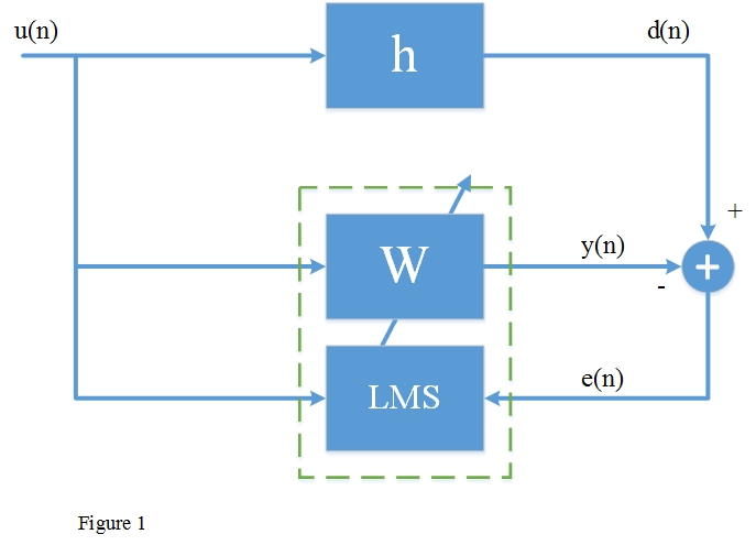
Figure 1 shows an adaptive filter structure that can be used for system identification or modeling. The same input u is to an unknown system in parallel with an adaptive filter. The error signal e is the difference between the response of the unknown system d and the response of adaptive filter y. The error signal fed back to the adaptive filter and is used to update the adaptive filter’s coefficients until the overall out y = d. When this happens, the adaptation process is finished, and e approaches zero.

Formulation
As you see in Figure 1, y (n) is the output of the adaptive filter:

Where w<sub>k</sub> (n) represent M weights or coefficients for a specific time n. The convolution equation can be implemented something like this:
for (int i = 0; i < M; i++)
Y += (W[i] * X[i]);
A performance measure is needed to determine how good the filter is. This measure is based on the error signal...

... which is the difference between desired signal d (n) and adaptive filters output y (n). The weights or coefficients wk (n) are adjusted such that a mean squared error function is minimized. This mean square error function is E [e<sup>2</sup> (n)], where E represents the expected value. Since there are k weights or coefficients, a gradient of the mean squared error function is required. An estimate can be found instead using the gradient of e<sup>2</sup> (n), yielding

That can be implemented like this:
E = D - Y;
for (int i = 0; i < M ; i++)
W[i] = W[i] + (mu * E * X[i]);
LMS Example in Code
We illustrate the following steps for the adaptation process using the adaptive structure in Figure 1:
- Generate some random data for LMS filter input.
- Assume a system that we are going to estimate it like this:
H[M] = { 1, 0.5, 0.25, 0.125, 0.0625 } - Build desired signal by convolving the generated random data and assumed
H. - Calculate the adaptive filter output
y. - Calculate the error signal
- Update each LMS filter weights
- Repeat the entire adaptive process for the next output sample point.
Generating Input and Desired Signals:
for (int i = 0; i < I; i++)
		Input[i] = rand() / (float)RAND_MAX;

	for (int i = 0; i < I; i++)
		for (int j = 0; j < M; j++)
			if (i - j >= 0)
				Desired[i] += Input[i - j] * H[j];
All Together
#define mu 0.2f //convergence rate
#define M 5 //order of filter
#define I 1000 //number of samples
double Input[I] = { 0.0 };
double Desired[I] = { 0.0 };
double H[M] = { 0.0625, 0.125, 0.25, 0.5, 1 };
void initialize()
{
for (int i = 0; i < I; i++)
Input[i] = rand() / (float)RAND_MAX;
for (int i = 0; i < I; i++)
for (int j = 0; j < M; j++)
if (i - j >= 0)
Desired[i] += Input[i - j] * H[j];
}
void main()
{
initialize();
long T, n = 0;
double D, Y, E;
double W[M] = { 0.0 };
double X[M] = { 0.0 };
FILE *Y_out, *error, *weights;
Y_out = fopen("Y_OUT", "w++"); error = fopen("ERROR", "w++"); weights = fopen("WEIGHTS", "w++");
for (T = 0; T < I; T++)
{
for (int m = T; m > T - M; m--){
if (m >= 0)
X[M + (m - T) - 1] = Input[m]; else break;
}
D = Desired[T]; Y = 0;
for (int i = 0; i < M; i++)
Y += (W[i] * X[i]);
E = D - Y;
for (int i = 0; i < M; i++)
W[i] = W[i] + (mu * E * X[i]);
fprintf(Y_out, "\n % 10g % 10f", (float)T, Y);
fprintf(error, "\n % 10g % 10f", (float)T, E);
}
for (int i = 0; i < M; i++)
fprintf(weights, "\n % 10d % 10f", i, W[i]);
fclose(Y_out);
fclose(error);
fclose(weights);
}
References
- The Adaptive Filters, Simon Haykin
- DSP Applications Using C and the TMS320C6x DSK
