Introduction
This article is written for you who is curious of the mathematics behind neural networks, NN. It might also be useful if you are trying to develop your own NN. It is a cell by cell walk through of a three layer NN with two neurons in each layer. Excel is used for the implementation.
Background
If you are still reading this, we probably have at least one thing in common. We are both curious about Machine Learning and Neural Networks. There are several frameworks and free api:s in this area and it might be smarter to use them than inventing something that is already there. But on the other hand, it does not hurt to know how machine learning works in depth. And it is also a lot more fun to explore things in depth.
My journey into machine learning has perhaps just started. And I started by Googling, reading a lot of great stuff on the internet. I also saw a few good YouTube videos. But I it was hard to gain enough knowledge to start coding my own AI.
Finally, I found this blog post: A Step by Step Backpropagation Example by Matt Mazur. It suited me, and the rest of this text is based on it.
Construction
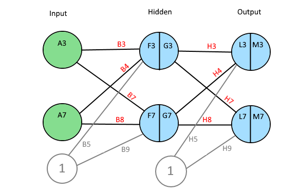
A Neural Network, NN, consists of many layers of neurons. A Neuron has a value and connections with weights to all other neurons in the next layer.
The first layer is the input layer and the last layer is the output layer. Between input and output, there might be one or many hidden layers. The number of neurons in a layer is variable.
If a NN is used to, for example, classify images, the number of neurons in the input layer is of course equal to the number of pixels in the image. Then in the output, each neuron represents a classification of the image. (E.g., a type of animal, a flower or a digit.)
Calculations
Before the calculations, all the weights in the NN have to be initialized with random numbers.
The image below is a print screen of the spread sheet that I refer to in the rest of this article. It might be a good idea to keep an open window of that sheet. That should make it easier to follow along.
A tip: Row 2 is the order of calculations.

Step 1 - 3. Forward Pass
The value of one neuron is calculated by taking the sum of every previous neuron multiplied by its weight.
An extra bias weight which has no neuron is also added:
F3 = A3 * B3 + A7 * B4 + B5
The value is normalized through a activation function. There are several different activation functions used in neural networks.
I have used the logistic function:
G3 = 1 / (1 + EXP(-F3))
Step 4 - 5. Forward Pass
The neurons of the output layer is calculated the same way as hidden layer.
L3 = G3 * H3 + G7 * H4 + H5
and
M3 = 1 / (1 + EXP(-L3))
Step 6 - 7. The Error
The error of each output neuron is calculated using an expected or a target value. When classifying images, it is common to set one neuron close to 1 and the rest of the neurons close to zero.
For the errors in column Q:
Q3 = (M3 - O3)²
and:
Q7 = (M7 - O7)²
The total Error R5 is the average of all errors and should get closer and closer to zero as the network is trained.
R5 = (Q3 + Q7) / 2
Backward Propagation
A Neural Network is trained by passing it lots of train data repeatedly.
Then, for every iteration, errors and deltas are calculated. This is used to make small adjustments to all the weights in such a way that the network becomes better and better.
This is called backpropagation.
Since the total error can be expressed as a mathematical functions of each weight, one can derive those functions to obtain the slopes of the function curves in one point. The slopes indicate the direction towards a minimum for the total error and proportionally how much each weight should be adjusted in order for the total error to approach zero.
A delta value is calculated below for each weight. The deltas are stored in column I and D, for output and hidden layer respectively.
Chain Rule - Friend of Backpropagation
In practice, we want to derive the total error R5 with respect to H3 so we first to express R5 as a function of H3 using substitutions.
Since
R5 = (Q3 + Q7) / 2
R5 = (M3 - O3)² / 2 + (M7 - O7)² / 2
The above function does not look very easy to derive. Is it even possible?
We will instead use the chain rule2.
It states that if we have a composition of two or more functions f(g(x)) and let F(x) = f(g(x)), we can derive like this:
F’(x) = f’(g(x)) * g’(x) or in another notation:
In our case, we have the following dependency:
R5(M3(L3(H3))) and we can write:
Step 9. Output layer Deltas
The function for the total error R5 is derived with respect to the first weight H3 of the output layer.
In the above formula, the chain rule is used to make it simpler to derive.
Since:
Proof of derivation of Logistic function found in this article3.
Since will be used later in the backpropagation, it is stored in the cell P3.
P3 = (M3-O3) * M3 * (1 - M3)
The last derivative of the chain of derivatives above is simpler.
Since L3 = G3 * H3 + G7 * H4 + H5
We can now put everything together and store into cell I3.
I3 = P3 * G3
The rest of the weights in output layer is calculated the same way and we get:
P7 = (M7-O7) * M7 * (1 - M7)

I4 = G7 * P3
I5 = 1 * P3 (bias neuron)
I7 = G3 * P7
I8 = G7 * P7
I9 = 1 * P7 (bias neuron)
Step 10. Backpropagation in Hidden Layer
In this step, we calculate:
The chain rule from previous steps helps to transform it to something we can use:
First term also must be split up on both errors Q3 and Q7 so:
First look at this:
It can be further split up like this:
First is already stored in P3 = (M3-O3) * M3* (1 - M3)
Since L3 = G3 * H3 + G7 * H4 + H5
When we put the above together, we get:
And in the same way as above:
First problem is solved.
Time for
We know that:
And we have previously learned to derive the logistic function.
And now:
Because:
We now put the above together to get one expression for the derivative of the total error with respect to first weight of the hidden layer.
This is stored in cell C3.
The calculations for the above is repeated for all hidden layer weights:
C3 = (P3 * H3 + P7 *H7) * (G3 *(1 - G3)) * A3
C4 = (P3 * H3 + P7 *H7) * (G3 *(1 - G3)) * A7
C5 = (P3 * H3 + P7 *H7) * (G3 *(1 - G3)) * 1
C7 = (P3 * H4 + P7 *H8) * (G7 *(1 - G7)) * A3
C8 = (P3 * H4 + P7 *H8) * (G7 *(1 - G7)) * A7
C9 = (P3 * H4 + P7 *H8) * (G7 *(1 - G7)) * 1
Now it is easy to calculate new weights using a selected learning rate from cell A13.
For example: (new B3)
D3 = B3 - C3 * A13
There is a macro connected to the train button in the Excel document. The macro iterates many times and we can see how the output neurons in column M gets closer and closer to their target values and that the total Error in R5 gets closer and closer to zero.
Update in version 1.1:
I discovered that it is possible to improve learning rate and accuracy by using the activation function Leaky Relu4:
f(x) = x if x > 0 otherwise f(x) = x/20
It may be a good exercise to replace the Logistic Function with Leaky Relu.
Hints:
G3 = IFS(F3 > 0; F3; F3 <= 0; F3/20)
and
P3= (M3-O3) * IFS(M3 > 0;1;M3<=0;1/20)
(Also attaching new version of the xls file, just in case...)
Final Words
I realize this article might take some time to digest. I tried to explain it as I understood it. Please comment below if you find any errors.
After I sorted out how NNs work in Excel, I wrote a C# program that can interpret hand written digits. It has a Windows Forms user interface which works well. It seems to recognize almost any digit I draw, even ugly once. That was a proof to me that my understanding of Artificial Neural Networks is correct so far.
That article can be found here:
Handwritten digits reader UI5
Links
- A Step by Step Backpropagation Example - Matt Mazur.
- Chain rule - Wikipedia
- Logistic function - Wikipedia
- Rectifier (neural networks) - Wikipedia
- Handwritten digits reader UI - Kristian Ekman
History
- 1st January, 2019 - Version 1.0
- 8th January, 2019 - Version 1.1
- Replaced Logistic activation function with LeakyReLu
- 11th January, 2019 - Version 1.2
- Update of names of biases in diagrams
- 23th Januray, 2019 - Version 1.3
- Changed du calculation to the total error to the average av errors

