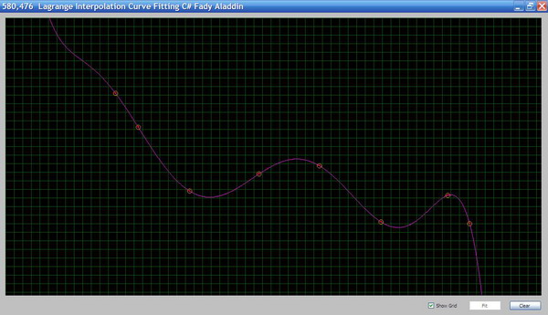
Introduction
In this article, I will explain curve fitting using the Lagrange interpolation polynomial. Curve fitting is used in a wide spectrum in engineering applications such as cars and air crafts surface design. The main problem is, given a set of points in the plan, we want to fit them in a smooth curve that passes through these points. The order of the curve f(x) depends on the number of points given. For example, if we have two points, the function will be of the first order, and the curve will be the line that passes through these two points, while if you have three points, the function will be of the second order f(x) = x2 . Let's first explain the Lagrange polynomial, then we will proceed to the algorithm and the implementation. In this article, I am using C# for coding.
Background
Lagrange Polynomial
An interpolation on two points, (x0, y0) and (x1, y1), results in a linear equation or a straight line. The standard form of a linear equation is given by y = mx + c, where m is the gradient of the line and c is the y-intercept.
m = y1 − y0 / x1 − x0
c = y0 − mx0
which results in:
y = (y1 − y0 / x1 − x0) * x + (x1 y0 − x0 y1 )/ (x1 − x0)
The linear equation is rewritten so that the two interpolated points, (x0, y0) and (x1, y1), are directly represented.
With this in mind, the linear equation is rewritten as:
P1(x) = a0(x − x1) + a1(x − x0)
where a0 and a1 are constants . The points x0 and x1 in the factors of the above equation are called the centers. Applying the equation at (x0, y0), we obtain:
y0 = a0(x0 − x1) + a1(x0 − x0)

or

a0 = y0/ x0−x1
At (x1, y1), we get:
y1 = a0(x1 − x1) + a1(x1 − x0), or a1 = y1/ x1−x0
Therefore, the linear equation becomes:
P1(x) = y0 (x− x1) /(x0 − x1) + y1 (x− x0) / (x1 − x0)
The quadratic form of the Lagrange polynomial interpolates three points, (x0, y0), (x1, y1), and (x2, y2). The polynomial has the form:
P2(x) = a0(x− x1)(x− x2) + a1(x− x0) (x− x2) + a2(x− x0)(x− x1)
with centers at x0, x1, and x2. At (x0, y0):
y0 = a0(x0 − x1)(x0 − x2) + a1(x0 − x0)(x0 − x2) + a2(x0 − x0)(x0 − x1),

or

a0 = y0/ (x0 − x1)(x0 − x2)
a1 = y1 / (x1 − x0)(x1 − x2)
a2 = y2/ (x2 − x0)(x2 − x1)
P2(x) = y0 (x− x1)(x− x2) / (x0 − x1)(x0 − x2) + y1 (x − x0)(x − x2)/
       (x1 − x0)(x1 − x2) + y2 (x− x0)(x− x1)/ (x2 − x0)(x2 − x1)
In general, a Lagrange polynomial of degree n is a polynomial that is produced from an interpolation over a set of points, (xi , yi ) for i = 0, 1, . . ., n, as follows:
Pn(x) = y0L0(x) + y1L1(x) + ··· + ynLn(x)
Using the Code
The Algorithm
Given the interpolating points (xi , yi ) for i =0, 1, . . . ,n;

for i = 0 to n
  //the cumulative multiplication from k = 1 (and k not equal i) to n
  Evaluate Li (x) = ∏nk=1,k != i (x−xk ) / (xi−xk ) ;
endfor

Evaluate Pn(x) = y0L0(x) + y1L1(x) + ··· + ynLn(x);
Download the source code from the top of this page to view the code.
Points of Interest
Numerical computing is a very interesting field in software development. This article is related to that field ... And, I will post more articles soon about Computational Geometry ...such as Convex Hull algorithm and Triangulation.
