Introduction
Let us understand FFT. It is Fast Fourier Transform, an
algorithm to calculate DFT or discrete fourier transform in fast and efficient
way. The first question that arises seeing the title is what the hell a
tutorial on FFT doing in the new article section of code project in the year
2012 when the algorithm is about 50 years old. Great Question. By the way, you can refer following links for understanding the same in a complicated way.
http://en.wikipedia.org/wiki/Discrete_Fourier_transform
http://en.wikipedia.org/wiki/Fast_Fourier_transform
Background
One of the reasons, I thought I must write this tutorial is
because I have seen many engineers finding it difficult to understand what
exactly is a frequency domain, what exactly is filtering. How can we filter a
signal in simple way. What is this symmetrical features of FFT and more
importantly understanding the core facts about FFT. So if you are a programming
Pro and a killer programmer having written your own DSP logics and algorithms,
then this article may not give you any new or interesting things. But if you
have just picked signal processing, you might find it quite helpful (Hopefully).
Using the Code
First Let us construct a simple sinusoidal signal of 50Hz
with amplitude=5. I am considering a sampling frequency of 100 times the
message frequency(it should it least be twice as par Nequist rate), which means
I will collect 1000 samples from the actual analog sinusoidal signal. So if the frequency is 50, that means you
will get one sample at 1/50 or .02 seconds. If you want 10 samples, you have to
gather the samples for .2 seconds. You will sample the signal at every 1/5000
seconds.
f=50;
A=5;
Fs=f*100;
Ts=1/Fs;
t=0:Ts:10/f;
x=A*sin(2*pi*f*t);
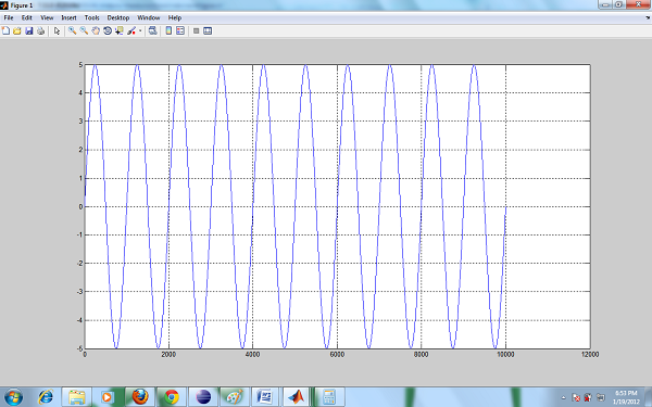
plot(x),grid on

Figure 1: Sinusoidal Signal of frequency 50Hz. Plot of Variable x.
So the figure shows 10 cycles of sine wave of 50 Hz. You can change the plot to stem type to see the samples.
So lets take FFT.
F=fft(x);
You must have studied about N point FFT. If you do not
specify N, then by default N is length of message signal. In this case it is
1001.
Very important thing: FFT divides your Sampling frequency
into N equal parts and returns the strength of the signal at each of these
frequency levels. What it means is you are dividing frequencies from 0 to 5000
into 1001 equal parts. So first point in
fft is 5Hz, next represents 10 Hz and so on. As the actual frequency of your
message is 50 Hz, you must get highest peak at that level. So let us plot FFT.
plot(real(F)),grid on

Figure 2: Plot of real part of the FFT output of signal x with highest peak marked. Plot of real part of Variable F.
What you see? The highest value is located at 11th position, which is nothing but 10th sample as matlab starts from 1.
10*5?=50Hz
It is so simple. But wait why do we get the imaginary part also? There is absolutely nothing called Imaginary values, they reflect past values.
Your signal is Sinusoidal, so you get negative cycle also right. Check this.
plot(real(imag(F))),grid on

Figure 3: Plot of imaginary part of the FFT output of signal x with highest peak marked. Plot of imaginary part Variable F.
what you see? :)
Yes the same thing with one negative amplitude peak also. I hope you get the idea.
Now let us understand how you can have some filtering with FFT. What I will do is mix couple of more signal with different frequency with same amplitude and same number of samples with your signal x.
x1=A*sin(2*pi*(f+50)*t);
x2=A*sin(2*pi*(f+250)*t);
x=x+x1+x2;

Figure 4: Plot of hybrid signal x containing 50Hz,100Hz,300Hz frequency components. Plot of Variable x.
Our signal now contains three components, a 50Hz,100Hz and 300Hz.
Its fft plot is the proof. Three frequencies at three levels, exactly at 50,100 and 300Hz.

Figure 5: Plot of real part of the FFT output of Hybrid signal x.
I want to recover my original signal. So if I keep the sample at 11th sample and leave the rest and then take ifft, I must get back my signal right. But the values of both 10th and 11th sample must be kept. It is called windowing.

Figure 6: Desired frequency band marked as a rectangular window in FFT plot of hybrid signal x .
See the red color window I have put over the FFT response of our Hybrid signal.
F2=zeros(length(F),1);
F2(10:11)=F(10:11);
xr=ifft(F2);
plot(real(xr)),grid on

Figure 7: Recovery of Original signal of Frequency component 50Hz from hybrid signal shown in figure 4, using rectangular window.
What you see? It is your original signal. But with less amplitude. This is because you choose a rectangular window and the loss is due to negative filter gain. You can now read a bit of digital filters and apply that.
Here is the complete code which may not be needed, but still I am posting it, in case you decide to spend some time and play with it.
 clear all;
clc;
close all
f=50;
 A=5;
Fs=f*100;
Ts=1/Fs;
t=0:Ts:10/f;
x=A*sin(2*pi*f*t);
x1=A*sin(2*pi*(f+50)*t);
x2=A*sin(2*pi*(f+250)*t);
x=x+x1+x2;
plot(x)
F=fft(x);
figure
N=Fs/length(F);
baxis=(1:N:N*(length(x)/2-1));
plot(baxis,real(F(1:length(F)/2)))
Points of Interest
You can learn Matlab fundamentals from this source <here>
To know the details about any Matlab command, you can simply click on that command in the editor and press F1. Matlab help file explains the usage and other details about the commands like fft,sin and so on.
Behind all that complicated mathematics, there is a simple logic. I love that simple logic really.
