Numerical Methods in C++ Part 2: Gauss-Legendre Integration

thoughts-on-coding

5.00/5 (3 votes)

25 Apr 2019CPOL2 min read

7.8K

Implementation of Numerical Integrations with Trapezoidal and Simpson Rule Approach.

Welcome back to a new post at thoughts-on-cpp.com. In this post, I would like to discuss the Gauss integration algorithm, more precisely the Gauss-Legendre integration algorithm. The Gauss-Legendre integration is the most known form of the Gauss integrations. Others are

Gauss-Tschebyschow
Gauss-Hermite
Gauss-Laguerre
Gauss-Lobatto
Gauss-Kronrod

The idea of the Gauss integration algorithm is to approximate, similar to the Simpson Rule, the function f(x) by

$f(x)=w(x) \cdot \phi (x)$

While w(x) is a weighting function, $\phi(x)$ is a polynomial function (Legendre-Polynomials) with defined nodes $x_i$ which can be exactly integrated. A general form for a range of a-b looks like the following.

$\int_{a}^{b} f(x) \mathrm{d} x \approx \frac{b-a}{2} \sum_{i=1}^{n} f\left(\frac{b-a}{2} x_{i}+\frac{a+b}{2}\right) w_{i}$

The Legendre-Polynomials are defined by the general formula and its derivative

$P_n(x)=\sum_{k=0}^{n/2}=(-1)^k\frac{(2n-2k)!}{(n-k)!(n-2k)!k!2^n}x^{n-2k}$

$P_{n}^{\prime}(x)=\frac{n}{x^{2}-1}\left(x P_{n}(x)-P_{n-1}(x)\right)$

The following image is showing the 3rd until the 7th Legendre Polynomials, the 1st and 2nd polynomials are just 1 and x and therefore not necessary to show.

First 5 Legendre Polynomials

Let’s have a closer look at the source code:

The integral is done by the gaussLegendreIntegral (line 69) function which is initializing the LegendrePolynomial class and afterward solving the integral (line 77 – 80). Something very interesting to note: We need to calculate the Legendre-Polynomials only once and can use them for any function of order n in the range a-b. The Gauss-Legendre integration is therefore extremely fast for all subsequent integrations.

The method calculatePolynomialValueAndDerivative is calculating the value (line 50) at a certain node $x_i$ and its derivative (line 51). Both results are used at method calculateWeightAndRoot to calculate the the node $x_i$ by the Newton-Raphson method (line 33 – 37).

$x_{n+1}=x_{n}-\frac{f\left(x_{n}\right)}{f^{\prime}\left(x_{n}\right)}$

The weight w(x) will be calculated (line 40) by

$w_{i}=\frac{2}{\left(1-x_{i}^{2}\right)\left[P_{n}^{\prime}\left(x_{i}\right)\right]^{2}}$

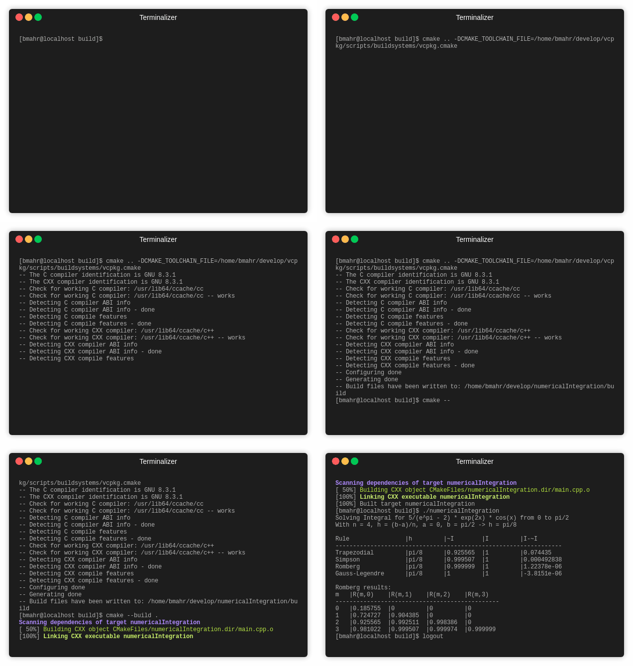
As we can see in the screen capture below, the resulting approximation of

$I=\int_0^{\pi/2} \frac{5}{e^\pi-2}\exp(2x)\cos(x)dx=1.0$

is very accurate. We end up with an error of only $-3.8151e^{-6}$ . Gauss-Legendre integration works very good for integrating smooth functions and result in higher accuracy with the same number of nodes compared to Newton-Cotes Integration. A drawback of Gauss-Legendre integration might be the performance in case of dynamic integration where the number of nodes are changing.

Screen capture of program execution

Did you like the post?

What are your thoughts?

Feel free to comment and share this post.

License

This article, along with any associated source code and files, is licensed under The Code Project Open License (CPOL)