The project can be compiled using qmake or through QtCreator. After starting the program, it will begin to work on the included sample image.
Introduction
Image segmentation is used in computer vision to locate objects boundaries. You can use it to precisely cut out objects from an image database (e.g. locating objects in satellite images) or if your algorithm is fast enough, it can be used in real-time like in robotics application.
The goal of object segmentation is to find a boundary between two zones: an object and its background. To be useful, we want the boundary to have properties similar to how we would cut out the object. That's why we have to use an algorithm which try to find simple boundaries without cutting uniform surface.
Algorithm
It was proved that solving the minimal cut problem is equivalent to finding the maximum amount which can flow from source to sink. Indeed this maximum flow will saturate the network at the same edge which is cut by the minimal cut. There are many algorithms from the combinatorial optimization domain which solve the maximum flow problem and thus our problem. The variant presented here is tuned to solve the problem on practical graphs from computer vision. It uses the fact that our graph is regular, each node is a pixel with only four neighbors.
Here is the outline of the algorithm:
The edge capacities are initialized from the difference between pixels. The algorithm then progresses in three step:
- Grow step: Active nodes (on the border of each tree) explore their neighboring and parent free nodes until they encounter a node from the other tree. When two nodes from opposite trees meet, they form a path.
- Augment step: We find the bottleneck along the found path and push the maximum flow through the path (i.e. subtract the maximum capacity from each edge capacity).
- Adoption step: Some edge will have been saturated, thus cutting parents from their children. These orphans try to find suitable parents in their neighbourhood. Parents can only adopt orphans from the same tree and if they are connected to their roots.
These steps are repeated until no more paths are found, meaning both search trees are cut from each other.
This pseudocode was extracted from the original algorithm description:
S={s}, T={t}, A={s,t}, O={}
loop
grow S or T to find an augmenting path P from s to t
if P = Ø terminate
augment on P
adopt orphans
while A = Ø {
pick an active node p ? A
for every neighbor q such that tree cap(p ? q) > 0 {
if TREE(q) = Ø then add q to search tree as an active node:
TREE(q) := TREE(p), PARENT(q) := p, A := A ? {q}
if TREE(q) = Ø and TREE(q) = TREE(p) return P = PATH( s?t )
}
remove p from A
}
return P = Ø
find the bottleneck capacity ? on P
update the residual graph by pushing flow ? through P
for each edge (p, q) in P that becomes saturated {
if TREE(p) = TREE(q) = S then set PARENT(q) := Ø and O := O ? {q}
if TREE(p) = TREE(q) = T then set PARENT(p) := Ø and O := O ? {p}
}
while O = Ø {
pick an orphan node p ? O and remove it from O
foreach neighbour q {
if
- TREE(p) = TREE(q)
- capacity( q -> p ) > 0
- q is not orphan (mark node confirmed to be connected to source at a given stage)
- best "distance to source"
then
PARENT(p) = q
} else foreach neighbour q with TREE(q) = TREE(p) { if capacity( q -> p ) > 0: A << q
if parent( q ) = p: O << q; parent(q)=0;
}
TREE(p) = 0
}
Implementation
The graph data is stored in an array (exactly as an image). Nodes are accessed via a cursor class which proxy the private data. The algorithm is divided in three methods to allow user interaction while it executes. Each method is implemented as described above.
User Interface
Thanks to Qt's Graphics View Framework, it is easy to add a user interface to visualize how the algorithm works. You only need to create a new scene and an antialiased view.
scene = new QGraphicsScene();
view = new QGraphicsView(scene);
view->setRenderHint( QPainter::Antialiasing );
view->setViewport(new QGLWidget(QGLFormat(QGL::SampleBuffers)));
The scene is redefined from scratch at each iteration using new data.
scene->clear();
for(int y=0;y<graph- />h;y++) for(int x=0;x<graph- />w;x++) {
NodePrivate* data = graph->node(x,y).data;
const QColor nodeColor[3] = { QColor(Qt::black), QColor(Qt::red), QColor(Qt::blue) };
QPen pen(nodeColor[data->tree]);
if( !data->active ) pen.setStyle(Qt::DotLine);
scene->addEllipse(x,y,0.5,0.5,pen);
... }
view->fitInView(scene->sceneRect(), Qt::KeepAspectRatio );
Using fitInView, you can use arbitrarily sized images and they will always fit your screen. This is the main advantage of a scene-graph API compared to direct rendering.
Conclusion
This article shows the steps from an abstract algorithm description to its implementation. As it is easier to understand concepts you can see in action, it presents a graphic visualization of the algorithm working on sample images. Not only does it make it easier to understand, but it also helps debugging and improving the algorithm. Instead of just watching the trees fighting for pixels, you could now adapt this code to practical applications.
Screenshot
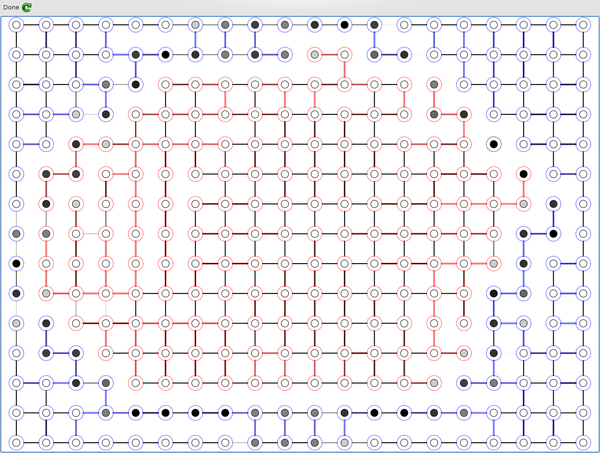
Each node represents one pixel of the image. Intensity is shown by the central circle value.
The colored nodes and edges represent the search trees: red for source and blue for sink.
The dotted nodes are passive nodes (i.e. inside the search tree) whereas the solid line nodes are active nodes (growing until a path is found).
The edge width represents the capacity. Saturated edges tend to disappear showing where the image might be cut.
Reference
- "An Experimental Comparison of Min-Cut/Max-Flow Algorithms for Energy Minimization in Vision", Yuri Boykov and Vladimir Kolmogorov, 2002
History
- 14th December, 2009: Initial post
This member has not yet provided a Biography. Assume it's interesting and varied, and probably something to do with programming.


 General
  News
News  Suggestion
  Question
  Bug
Bug  Answer
  Joke
Joke  Praise
  Rant
Rant  Admin
Admin 


