Introduction
Density-based spatial clustering of applications with noise(DBSCAN) is a clustering algorithm based on density. Unlike other clustering algorithms, DBSCAN regards the maximum set of density reachable samples as the cluster. KMeans lacks the ability to cluster the nonspherical data, while DBSCAN can cluster data with any shape.
DBSCAN Model
Preliminary
- ε -neighbor: Objects within a radius of ε from an object.
- Core point: One sample is a core point if it has more than a specified number of points (m) within ε- neighbor.
- Directly density-reachable: An object q is directly density-reachable from object p if q is within the ε-Neighborhood of p and p is a core object.
- Density-reachable: An object q is density-reachable from p if there is a chain of objects p1,…,pn, with p1=p, pn=q such that pi+1is directly density-reachable from pi for all 1 <= i <= n (the difference between Directly density-reachable and Density-reachable is that p is within the neighbor of q when Directly density-reachable while p is not within the neighbor of q when density-reachable)
- Density-connectivity: Object p is density-connected to object q if there is an object o such that both p and q are density-reachable from o
- Noise: objects which are not density-reachable from at least one core object
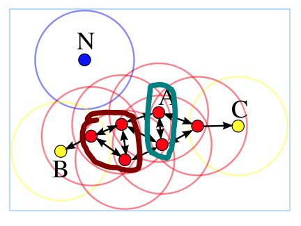
Let's give a example to explain the above terms as shown below, where m = 4. Because there are more than m samples in the ε- neighbors of all the red samples, they are all core points and density-reachable. B and C are not core points. The samples in the cyan circle are directly density-reachable. The samples in the brown circle are density-connectivity. N is not reachable to any other samples, thus it is a noise point.

Clustering Algorithm
First, we find all the core points by calculating the number of samples within all the samples ε- neighbor. The remained samples are marked noise point as temporarily. We provide several types of distance, namely:
- Euclidean distance:

- Cosine distance:

- Manhattan distance:

def calculateDistance(self, x1, x2):
if self.distance_type == "Euclidean":
d = np.sqrt(np.sum(np.power(x1 - x2, 2), axis=1))
elif self.distance_type == "Cosine":
d = np.dot(x1, x2)/(np.linalg.norm(x1)*np.linalg.norm(x2))
elif self.distance_type == "Manhattan":
d = np.sum(x1 - x2)
else:
print("Error Type!")
sys.exit()
return d
For a given sample, if the distance between this sample and another sample is less than ε, they are in the same neighbor.
def getCenters(self, train_data):
    neighbor = {}
    for i in range(len(train_data)):
        distance = self.calculateDistance(train_data[i], train_data)
        index = np.where(distance <= self.eps)[0]
        if len(index) > self.m:
            neighbor[i] = index
    return neighbor
Then, we choose an unvisited core point P randomly to merge the samples which are density-connectivity with it. Next, we visit the samples Q within ε- neighbor of P. If Q is a core point, Q is in the same cluster of P and do the same process on Q (like depth first search); else, visit the next sample. Specifically, the search process in P's ε- neighbor is shown below:
- Choose core point A and find all the samples in its ε- neighbor. The samples within A's ε- neighbor belong to the cluster of A. Then visit the samples within A's ε- neighbor successively.

- Visit the sample B within A's ε- neighbor. B is a core sample, visit the samples within B's ε- neighbor.

- Visit the sample C within B's ε- neighbor. C belongs to A and C is not a core point. Visit the other samples within B's ε- neighbor.

- Visit another sample D within B's ε- neighbor. D is a core point. Visit the samples within D's ε- neighbor.

- Visit the sample E. E is not a core point. Now, there is not any point density-reachable to A. Stop clustering for A.

k = 0
unvisited = list(range(sample_num))
while len(centers) > 0:
visited = []
visited.extend(unvisited)
cores = list(centers.keys())
randNum = np.random.randint(0, len(cores))
core = cores[randNum]
core_neighbor = []
core_neighbor.append(core)
unvisited.remove(core)
while len(core_neighbor) > 0:
Q = core_neighbor[0]
del core_neighbor[0]
if Q in initial_centers.keys():
diff = [sample for sample in initial_centers[Q] if sample in unvisited]
core_neighbor.extend(diff)
unvisited = [sample for sample in unvisited if sample not in diff]
k += 1
label[k] = [val for val in visited if val not in unvisited]
for index in label[k]:
if index in centers.keys():
del centers[index]
Parameter Estimation
DBSCAN algorithm requires 2 parameters ε, which specify how close points should be to each other to be considered a part of a cluster; and m, which specifies how many neighbors a point should have to be included into a cluster. Take an example from wiki, we calculate distance from each point to its nearest neighbor within the same partition as shown below, we can easily determine ε = 22.

For parameter m, we calculate how many samples are within core point's ε neighborhood as shown below. We choose m = 129 because it is the first valley bottom.

Conclusion and Analysis
DBSCAN has the ability to cluster nonspherical data but cannot reflect high-dimension data. When the density is not well-distributed, the clustering performance is not so good. The clustering performance between KMeans and DBSCAN is shown below. It is easy to find that DBSCAN has better clustering performance than KMeans.


The related code and dataset in this article can be found in MachineLearning.
