Recursion and Backtracking

Recursion

The simplest recursion function with practical use that I can come up with, is the factorial function.
The factorial is the result of all integer numbers below it multiplied together with itself.
Example: factorial to 4! = 4*3*2*1 = 24

def factorial(n):
  if(n>1):
    return factorial(n-1) * n
  return 1

This Python sample takes the factorial to a given value, by calling itself recursively.

The "n" value as input is subtracted by 1 in each recursive call, resulting in “n” becoming 0, and full depth of the recursion is reached, thus outputting the factorial value.

I’m not saying this is the best way to solve this problem. This could easily be resolved with less code without recursion.

Here is another recursion sample calculating pi using the Nilakantha series.

def CalcPiDecimals(opr,preciciendept):
  if preciciendept < 1:
    return 0
  preciciendept -= 1
  return 4/(opr * (opr + 1) * (opr + 2)) - 4/((opr + 2) * (opr + 3)* (opr + 4)) + 
            CalcPiDecimals(opr + 4,preciciendept)

print(3 + CalcPiDecimals(2,500))

Here, the recursion function only calculates the decimal part of the value. 3 needs to be added to the result.
This function, with this dept, outputs 3.141592653340542.

Backtracking

You can make recursion even more awesome by using backtracking to explore different solutions and options.

This sample is inspired by a video from the Youtube channel Computerfile.

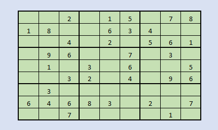
Here is a typically Sudoku, let's solve that.

import numpy as np

#Converted to numpy array
sudoku = np.array([[0, 0, 2, 0, 1, 5, 0, 7, 8],
                   [1, 8, 0, 0, 6, 3, 4, 0, 0],
                   [0, 0, 4, 0, 2, 0, 5, 6, 1],
                   [0, 9, 6, 0, 0, 7, 0, 3, 0],
                   [0, 1, 0, 3, 0, 6, 0, 0, 5],
                   [0, 0, 3, 2, 0, 4, 0, 9, 6],
                   [0, 3, 0, 0, 0, 0, 0, 0, 0],
                   [6, 4, 9, 8, 3, 0, 2, 0, 7],
                   [0, 0, 7, 0, 0, 0, 0, 1, 0]
                   ])

# test if a value on a specific place is possible with current data
def possible(sudoku,rov, col, val):
    if sudoku[rov][col] != 0:
        return False #Already filled
    if val in sudoku[rov]:
        return False #Value already in row
    for a in range(9):
        if sudoku[a][col] == val:
            return False #value already in column
    sqrov = int(int(rov) / 3) * 3
    sqcol = int(int(col) / 3) * 3
    for r in range(sqrov, sqrov + 3):
        for c in range(sqcol, sqcol + 3):
            if sudoku[r][c] == val:
                return False #value already in square
    return True  # Value possible

#solve a sudoku if possible, Fill out list
def solve_Sudoku(sudoku):
    for rov in range(0, 9):
        for col in range(0, 9):
            if sudoku[rov][col] == 0:
                for val in range(1, 10):
                    if possible(sudoku,rov, col, val):
                        sudoku[rov][col] = val
                        if solve_Sudoku(sudoku):
                            return True
                        sudoku[rov][col] = 0 #Backtrack
                return False #Solution failed, backtrack for next value
    return True

solve_Sudoku(sudoku)
print(sudoku)

In this sample, the exiting things is happening in the “Solve” function.

The “possible” function just checks any value for obeying the sacred rules of Sudoku.

You know:

• Only values between 1 and 9 can be used
• Only one occurrence of a value in each row
• Only one occurrence of a value in each column
• Only one occurrence of each value in one square when the sudoku plate is divided into nine squares

The “solve” function iterates through each row and each column in the sudoku array, looking for an unsolved field (containing 0). When found, it's iterating through possible values. Trying each value with the “Possible” function, until “possible” return True.

If the “Possible” function returns true, the value is kept in the sudoku array, and the “Solve” function is recursively called to iterate to the next Row/column with unsolved value. This is illustrated with green arrows below.

Maybe not the best illustration in the world, but making it helped me understand the whole thing better, which is the main point of this article.

If the “possible” function returns False, the sudoku array field is marked unsolved again, and the loop looks for the next value to try in the field. If no value for a field could fulfill the rules of sudoku, the backtracking begins.

The red arrow in the illustration show that a False result from the possible function resolves in the value in the sudoku array is erased (backtracked), and the loop continues to the next value. This backtracking can go multiple steps backwards until the “possible” function starts returning True again. Then the recursion moves forward shown with green arrows.

When the row and col loop reach the end, the sudoku is solved if possible, and “solve” function returns true all the way through the call stack, until it reaches the entry point. The blue arrows.

See the whole illustration here.

The solved sudoku is printed.

[[9 6 2 4 1 5 3 7 8]
 [1 8 5 7 6 3 4 2 9]
 [3 7 4 9 2 8 5 6 1]
 [4 9 6 1 5 7 8 3 2]
 [2 1 8 3 9 6 7 4 5]
 [7 5 3 2 8 4 1 9 6]
 [5 3 1 6 7 2 9 8 4]
 [6 4 9 8 3 1 2 5 7]
 [8 2 7 5 4 9 6 1 3]]

I began to write a maze solving algorithm with backtracking, but realized that computerfile already did a video on that, end I wouldn’t be able to make mine as effective as theirs, without any optimizing features.

So instead, I will just link to the computerfile video. Maze solving.

It’s a really nice channel, and Mike Pound, and other guests really know their stuff.

Hope you have fun coding, and enjoyed reading my article.

History

• 18^th March, 2020: Initial version