Here we look at: Minimizing Jitter, and parameter grid search with an example of doing a simple grid search.
In the previous articles of this series, we tried the various approaches to learning the OpenAI Gym Atari Breakout environment, both from pixels and from the contents of its RAM.
Now we will explore a couple of advanced Breakout learning topics.
Minimizing Jitter
Araty Breakout agents do not play very smoothly. For example, it is common for the bat to "jitter" back and forth for no clear reason.
In this section, we will try to minimize this unnecessary movement by penalizing the agent for performing it.
Here is the code I used:
import gym
import ray
from gym import Wrapper
from ray import tune
from ray.rllib.agents.impala import ImpalaTrainer
from ray.tune.registry import register_env
ray.shutdown()
ray.init(include_webui=False, ignore_reinit_error=True)
class PenaliseMovement(Wrapper):
def __init__(self, env):
super().__init__(env)
self._call_count = 0
def step(self, action):
observation, reward, done, info = super().step(action)
if reward > 1.0:
reward = 1.0
threshold = 375_000
if self._call_count >= threshold and action not in (0, 3):
multiplier = min((self._call_count - threshold) / 100_000, 1.0)
reward -= 0.0001 * multiplier
self._call_count += 1
return observation, reward, done, info
def env_creator(env_config):
env = gym.make('BreakoutNoFrameskip-v4')
env = PenaliseMovement(env)
return env
register_env("penalise_movement_breakout", env_creator)
ENV = "penalise_movement_breakout"
TARGET_REWARD = 200
TRAINER = ImpalaTrainer
tune.run(
TRAINER,
stop={"episode_reward_mean": TARGET_REWARD},
config={
"env": ENV,
"monitor": True,
"evaluation_num_episodes": 25,
"rollout_fragment_length": 50,
"train_batch_size": 500,
"num_workers": 7,
"num_envs_per_worker": 5,
"clip_rewards": False,
"lr_schedule": [
[0, 0.0005],
[20_000_000, 0.000000000001],
],
}
)
This uses an environment wrapper that is set to introduce a small negative reward for each action that is neither NO-OP (0) nor FIRE (3). The learning challenge is harder because the negative reward for moving is delivered immediately, whereas the positive reward for knocking out a brick is applied sometime after the action of the ball bouncing off the bat.
I got the best result by waiting for the learner to get a grip on the standard environment before introducing the penalty (threshold in the code above), and then introducing the penalty over 100,000 steps instead of all at once. This is a form of curriculum learning. Learning these two regimes separately is a lot easier than conflating them from the start.
The penalty size is important: too small and it will not have any effect; too large and the agent might just learn to stand still. What we want is just enough of a nudge to act as a dampening factor.
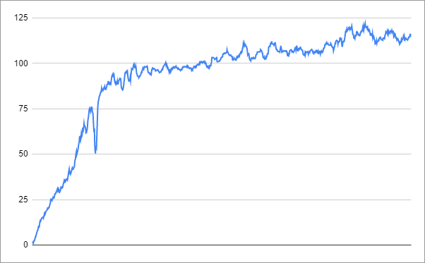
The performance graph looked like this (note that it is no longer meaningful to compare these rewards with the standard environment directly):

When the score reaches about 80, the more complex reward structure is introduced, and the rate of learning decreases.
The agent reached the performance of 116 after 3.6 hours, when I stopped the process. Whether it was actually smoother is open to debate. I’d be interested to hear in the comments if you have any success with this approach.
Parameter Grid Search
We have been using RLlib’s tune function throughout this series as a convenient way to run the training, but without using it for actually tuning the parameters.
Here is an example of doing a simple grid search. It sets up a tuning session on the cartpole environment as follows (the letters refer to code lines):
- Run each training session for five iterations (A)
- Search across three candidates for the learning rate (B)
- Search across three candidates for the hidden layer architecture of the neural network (C)
- Run each trial twice to counteract sensitivity to the initial state of randomness (D)
import ray
from ray import tune
from ray.rllib.agents.dqn import DQNTrainer
ray.shutdown()
ray.init(
include_webui=False,
ignore_reinit_error=True,
object_store_memory=8 * 1024 * 1024 * 1024
)
ENV = 'CartPole-v0'
TRAINER = DQNTrainer
analysis = tune.run(
TRAINER,
stop={"training_iteration": 5},
config={
"env": ENV,
"num_workers": 0,
"num_gpus": 0,
"monitor": False,
"lr": tune.grid_search([0.001, 0.0003, 0.0001]),
"hiddens": tune.grid_search([[256], [128], [200, 100]])
},
num_samples=2,
)
print("Best config: ", analysis.get_best_config(metric="episode_reward_mean"))
df = analysis.dataframe()
print(df)
When I ran this, the result was as follows:
Best config: {'env': 'CartPole-v0', 'num_workers': 0, 'num_gpus': 0, 'monitor': False, 'lr': 0.0003, 'hiddens': [256]}
which tells us that a learning rate of 0.0003 and a hidden layer configuration of [256] are good choices for performing best over five iterations, and that they are promising settings for training the model to completion.
To see all the available metrics for get_best_config, see the columns of the dataframe:
print(df.columns)
To find good candidate parameters to search over, the following might be helpful. For RLlib there are two complementary sets of "known good" settings for learning different environments:
- The tuned_examples directory in RLlib itself. It focuses on sensible working parameters for the various environments.
- A separate repository in the Ray project called rl-experiments. There you will find reference results for comparing against the performances published in the scientific papers.
For each algorithm, both sources suggest a single set of Atari game parameters. If you want a challenge, investigate whether you can find better parameters that work well for specific environments.
Grid searching is an expensive exercise, especially in environments more challenging than the cartpole. The search space quickly adds up to require a very large number of trials. This is sometimes referred to as the curse of dimensionality.
I hope you have enjoyed this introduction to reinforcement learning, and that it encouraged you to do some experimentation on your own. I look forward to reading any questions or suggestions in the comments.
