This article shows the code to create and train a model using TensorFlow and then run model training on Azure ML. This will be followed by a brief demonstration to show that the trained model works as expected.
In this series, we work through several approaches to creating and using machine learning models in Python on Azure. In the first article, we used Visual Studio Code with ML extensions to train an XGBoost model on Azure. Then, we used GitHub Codespaces and GitHub Actions to automatically train a PyTorch model after each push of changes to a repository.
In most real-life machine learning projects, the actual training of the final model requires a long experimentation phase. This phase is highly interactive, so using regular Python code alone is uncommon. Initially, you’ll use mostly the Jupyter notebook on JupyterLab. This article shows how to train within an Azure Machine Learning workspace using a TensorFlow model.
You can find the sample code for this article on GitHub.
Prerequisites
To follow examples from this article, you need a web browser and access to an Azure subscription. If you don’t have a subscription, you can sign up for a free Azure account.
Setting Up the Azure Machine Learning Workspace
If you have followed examples in the previous two articles, you should already have an Azure: Machine Learning workspace created. If not, you can quickly build it the same way as any other Azure resource. One way to do it is to log in to the Azure Portal, click Create a Resource, then type "machine learning" into the search box.
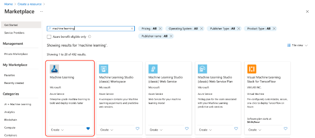
After selecting Machine Learning from the list and clicking Create, you need to enter your workspace’s details.
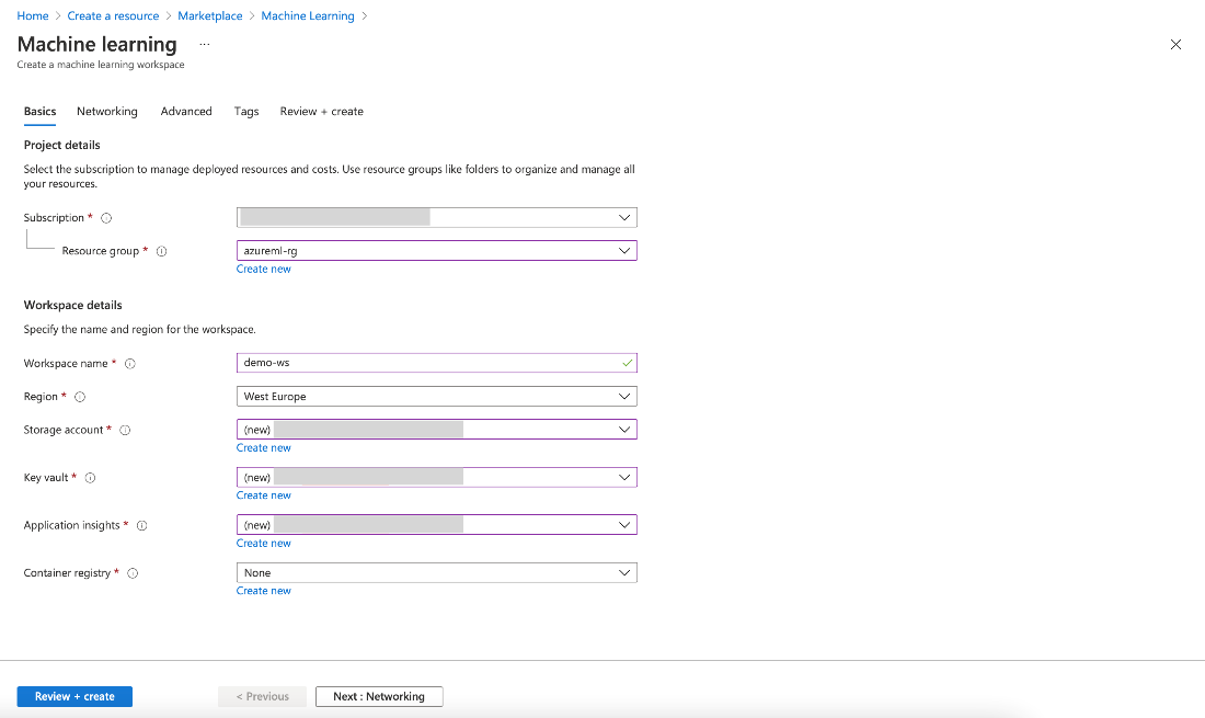
You can enter any values you like, but we refer to azureml-rg as our resource group and demo-ws as the workspace name in the following examples. When satisfied, click Review + create, then click Create on the final wizard screen. After a few minutes, you have access to your new resource.
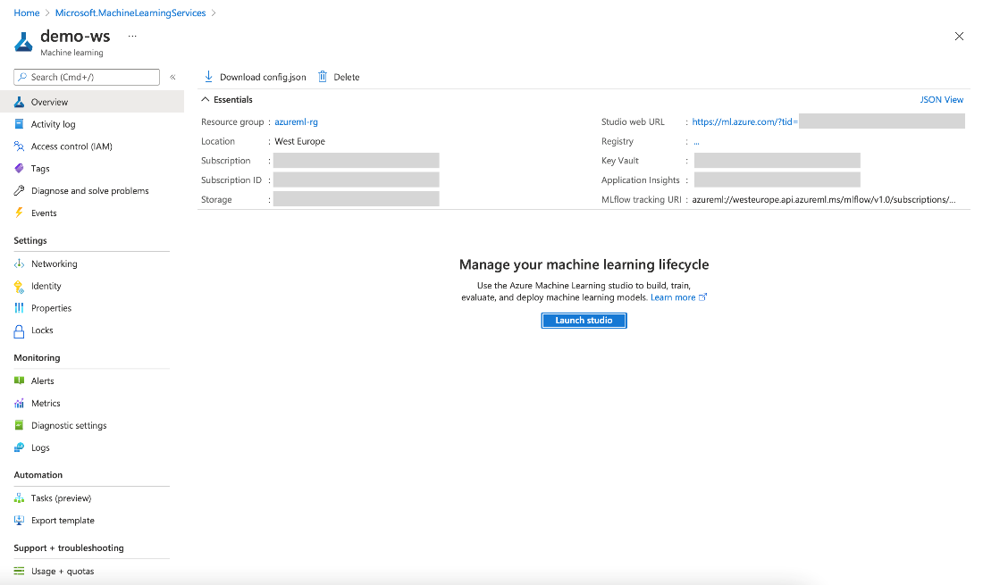
The rest of the time we spend in the Azure Machine Learning Studio. To get there, click Launch studio in the Azure portal or enter ml.azure.com manually in the browser. Then, select your workspace.
Preparing the Azure ML Notebook
The easiest way to create a notebook is by clicking the Start now button in the Azure Machine Learning Studio’s Notebooks tile:
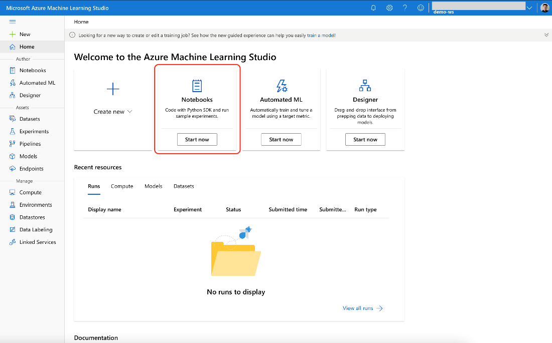
Before that, we need to add a compute. Without it, we can still create and edit a notebook but not run its code.
To continue, click the Compute option on the left-side menu.
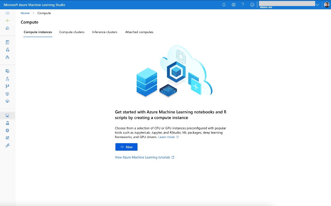
Here, we have four options to choose from:
- Compute instances
- Compute clusters
- Inference clusters
- Attached computers
The compute instance is the best choice for working with notebooks.
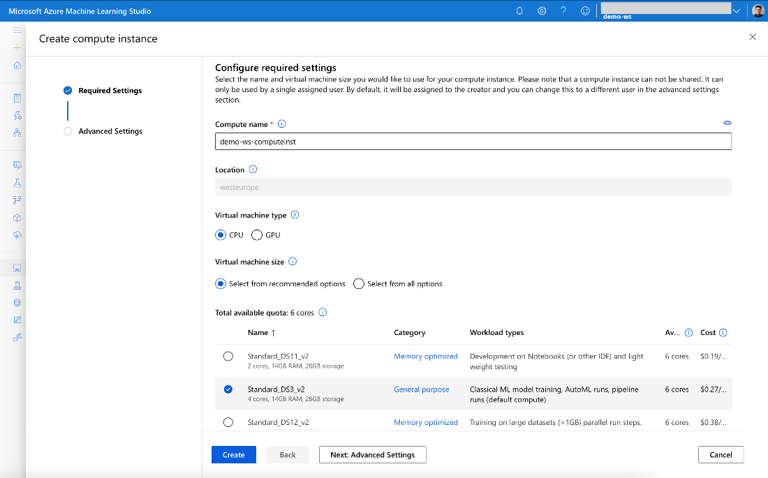
When creating a new compute instance, we need to provide its name and virtual machine (VM) parameters. You may need to be a little creative here, as it must be unique in your Azure region. If you expect heavy calculations, you may consider a VM with GPU.
Unlike compute clusters used for background processing, provisioning the compute instance when needed and deleting it when not used isn’t automatic. Initially, you spend most of your time writing the code, not running it. So, the GPU would be idle anyway.
When the compute is running, you see its status on the Compute instances tab:
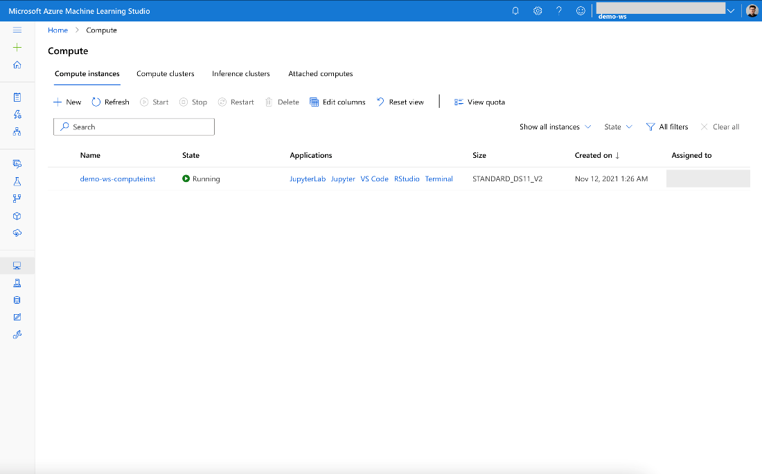
From here, we can start either JupyterLab or Jupyter. Select whichever option you prefer. It doesn’t matter for our purposes, so we continue with Jupyter. For more serious development, JupyterLab provides many helpful features, though.
When Jupyter starts, which should take only a moment, we select New, then the Python 3.8 - Tensorflow kernel. We end up with a new, empty notebook.
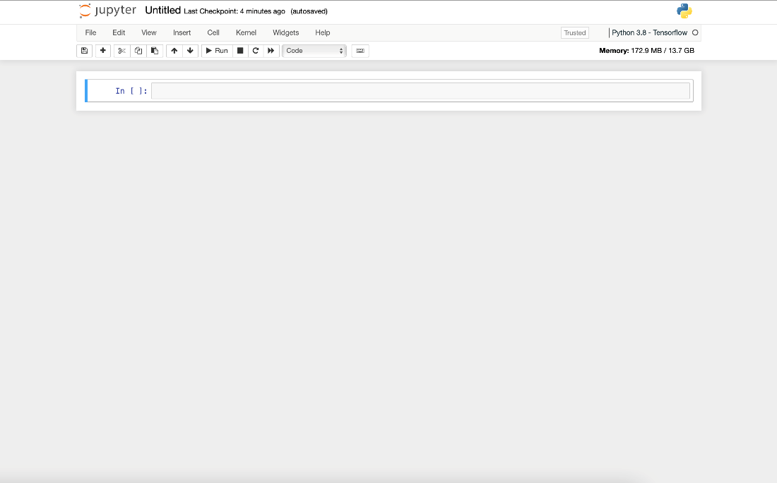
Let’s name it (for example, “aml-demo-tf-notebook”). Now we’re ready to start.
Downloading an MNIST Dataset
As in the previous two articles in this series, we start by downloading the MNIST handwritten digits dataset. We use Microsoft’s Azure Open Datasets as a source:
import os
import urllib.request

DATA_FOLDER = os.path.join(os.getcwd(), 'datasets/mnist-data')
DATASET_BASE_URL = 'https://azureopendatastorage.blob.core.windows.net/mnist/'
os.makedirs(DATA_FOLDER, exist_ok=True)

urllib.request.urlretrieve(
os.path.join(DATASET_BASE_URL, 'train-images-idx3-ubyte.gz'),
filename=os.path.join(DATA_FOLDER, 'train-images.gz'))
urllib.request.urlretrieve(
os.path.join(DATASET_BASE_URL, 'train-labels-idx1-ubyte.gz'),
filename=os.path.join(DATA_FOLDER, 'train-labels.gz'))
urllib.request.urlretrieve(
os.path.join(DATASET_BASE_URL, 't10k-images-idx3-ubyte.gz'),
filename=os.path.join(DATA_FOLDER, 'test-images.gz'))
urllib.request.urlretrieve(
os.path.join(DATASET_BASE_URL, 't10k-labels-idx1-ubyte.gz'),
filename=os.path.join(DATA_FOLDER, 'test-labels.gz'))
After executing this cell, the dataset files will be ready to use.
Exploring the MNIST Dataset
With the dataset downloaded to our ML workspace, we can explore it. First, we need to load it. This part of the code is dataset-specific and, in our case, is borrowed from the Azure Open Datasets example. If you’d like to use your data, you need to update or replace it accordingly.
import gzip
import struct
import numpy as np

def load_dataset(dataset_path):
def unpack_mnist_data(filename: str, label=False):
with gzip.open(filename) as gz:
struct.unpack('I', gz.read(4))
n_items = struct.unpack('>I', gz.read(4))
if not label:
n_rows = struct.unpack('>I', gz.read(4))[0]
n_cols = struct.unpack('>I', gz.read(4))[0]
res = np.frombuffer(gz.read(n_items[0] * n_rows * n_cols), dtype=np.uint8)
res = res.reshape(n_items[0], n_rows * n_cols) / 255.0
else:
res = np.frombuffer(gz.read(n_items[0]), dtype=np.uint8)
res = res.reshape(-1)
return res

X_train = unpack_mnist_data(os.path.join(dataset_path, 'train-images.gz'), False)
y_train = unpack_mnist_data(os.path.join(dataset_path, 'train-labels.gz'), True)
X_test = unpack_mnist_data(os.path.join(dataset_path, 'test-images.gz'), False)
y_test = unpack_mnist_data(os.path.join(dataset_path, 'test-labels.gz'), True)

return X_train.reshape(-1,28,28,1), y_train, X_test.reshape(-1,28,28,1), y_test
Apart from simply loading the data, the load_dataset method normalizes pixel values (from range 0-255 to 0-1) and shapes the output into dimensions expected by the TensorFlow framework.
To load our dataset, we run:
X_train, y_train, X_test, y_test = load_dataset(DATA_FOLDER)
We can confirm that we have expected 60,000 monochromatic images in the training set (28 x 28 pixels each):

Let’s check what’s in there:
def show_images(images, labels):
images_cnt = len(images)
f, axarr = plt.subplots(nrows=1, ncols=images_cnt, figsize=(16,16))
for idx in range(images_cnt):
img = images[idx]
lab = labels[idx]
axarr[idx].imshow(img, cmap='gray_r')
axarr[idx].title.set_text(lab)
axarr[idx].axis('off')

plt.show()

show_images(X_train[:10], y_train[:10])
Running this cell will show us the first ten labeled images from the training set:

Defining the Model
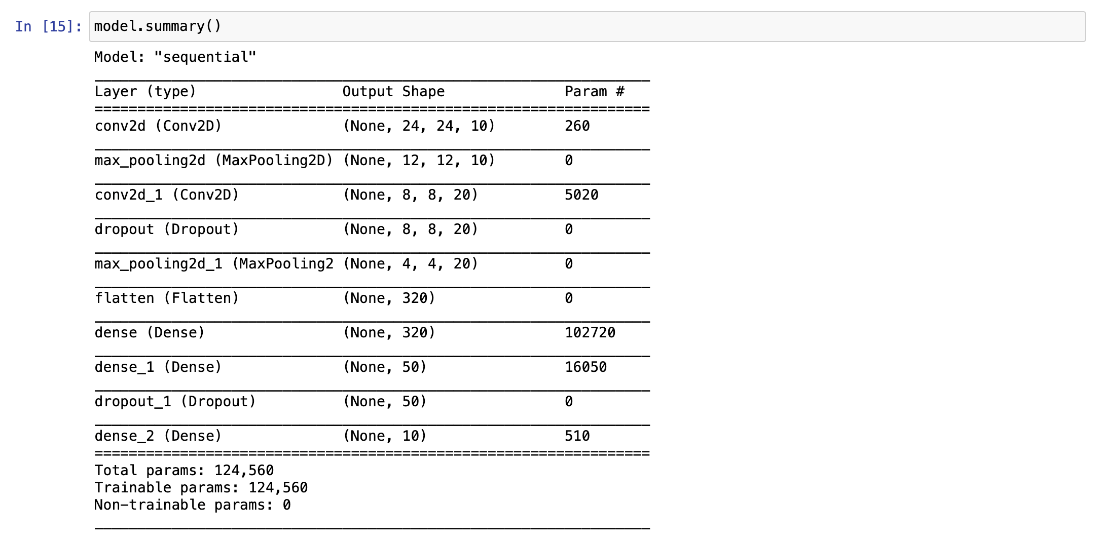
We have data, so now we can start working on the model. To keep things fit-to-purpose, we’ll create a simple convolutional neural network (CNN), which accepts a 28 x 28 matrix, and returns the probability score for each of 10 digits.
import tensorflow as tf
def create_tf_model():
model = tf.keras.models.Sequential(
[
tf.keras.layers.Conv2D(filters=10, kernel_size=5, input_shape=(28,28,1), activation='relu'),
tf.keras.layers.MaxPool2D(pool_size=(2,2)),
tf.keras.layers.Conv2D(filters=20, kernel_size=5, activation='relu'),
tf.keras.layers.Dropout(rate=0.2),
tf.keras.layers.MaxPool2D(pool_size=(2,2)),
tf.keras.layers.Flatten(),
tf.keras.layers.Dense(320, activation='relu'),
tf.keras.layers.Dense(50, activation='relu'),
tf.keras.layers.Dropout(0.2),
tf.keras.layers.Dense(10, activation='relu')
]
)
return model

model = create_tf_model()
model.build()
Using the model.summary method, we can inspect its layers and number of parameters:
Training the Model
Before training, we must compile our model with a selected loss function and optimizer:
loss_fn = tf.keras.losses.SparseCategoricalCrossentropy(from_logits=True)
model.compile(optimizer="adam", loss=loss_fn, metrics=["accuracy"])
Now, we can start the training. If we want to keep our training history in the Azure ML experiments, we need to take care of it first:
from azureml.core import Workspace, Experiment
import mlflow, mlflow.tensorflow
SUBSCRIPTION="<your-subscription-id>"
GROUP="azureml-rg"
WORKSPACE="demo-ws"

ws = Workspace(
subscription_id=SUBSCRIPTION,
resource_group=GROUP,
workspace_name=WORKSPACE,
)
experiment = Experiment(ws, "aml-demo-tf-notebook-training")

mlflow.set_tracking_uri(ws.get_mlflow_tracking_uri())
mlflow.start_run(experiment_id=experiment.id)
mlflow.tensorflow.autolog()
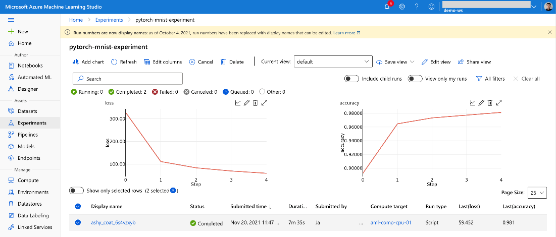
Using the code above, we create the new experiment (aml-demo-tf-notebook-training), inform the MLflow framework to use the Azure ML workspace for tracking, start a new run, and finally ask MLflow to log the TensorFlow training progress automatically. This auto-logging feature ensures model parameter and training progress tracking without additional manual steps.
With all these pieces in place, we can finally start the training. To ensure repeatable results between runs, we use a constant random feed:
tf.random.set_seed(101)
model.fit(X_train, y_train, epochs=5)
mlflow.end_run()
Our simple model and relatively simple dataset shouldn’t take long regardless of the selected compute instance VM’s size.

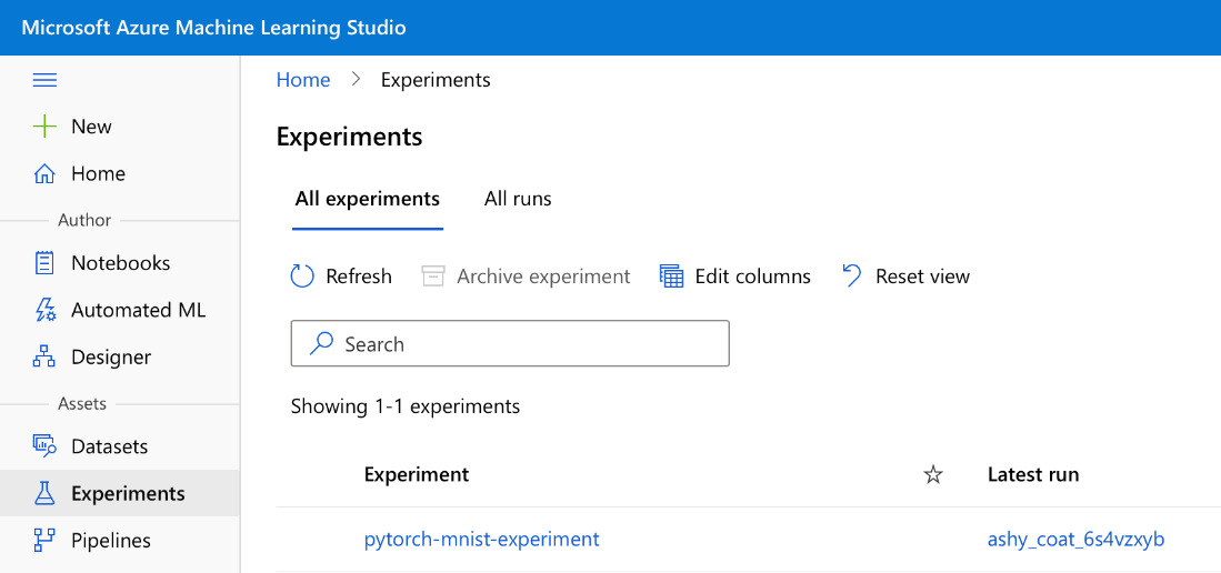
Thanks to our tracking configuration, we can check its progress and metrics using the Experiments tab in Machine Learning Studio (both during and after the training):
If training your model takes too long, it may be the moment to reconsider the compute VM’s size. At any time, you can go back to the Compute section of Machine Learning Studio to create a more powerful VM instance, then re-run the notebook. Alternatively, you can save the training code in a separate file and run the training on a compute cluster. The latter is slightly easier to do using Visual Studio Code, as shown in the previous two articles.
Evaluating and Registering the Model
After the training, we can check how our model works on the previously unseen test data. The simplest way is by using the model’s evaluate method:

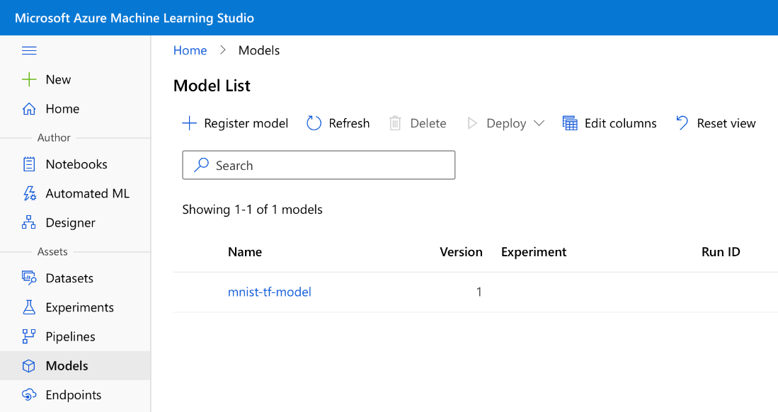
We have 98 percent accuracy. If the model is good enough for us, we can save it and register for future use. There are multiple options to save a TensorFlow model. We use the single-file HDF5 format for its portability. Finally, after saving the model, we can register it in the Azure: Machine Learning workspace:
from azureml.core.model import Model
model.save(‘mnist-tf-model.h5')
registered_model = Model.register(
workspace=ws,
model_name='mnist-tf-model',
model_path='mnist-tf-model.h5',
model_framework=Model.Framework.TENSORFLOW,
model_framework_version=tf.__version__)
The trained model is now available for future use.
Using the Saved Model for Predictions
To load the model registered in the Azure: Machine Learning workspace, we use the following code:
aml_model = Model(workspace=ws, name='mnist-tf-model', version=registered_model.version)
downloaded_model_filename = aml_model.download(exist_ok=True)
downloaded_model = tf.keras.models.load_model(downloaded_model_filename)
If you run this code in a different notebook session from the training, make sure to provide the correct value of the version parameter.
Let’s examine what we have loaded:
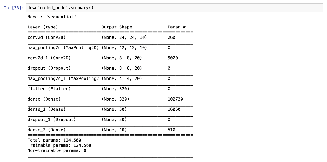
Now we can use the model for predictions.
preds = downloaded_model.predict(X_test).argmax(axis=1)
We can quickly check how it compares to our ground-truth:

As we can see, the first and the last three predicted values are correct.
If we still don't have confidence in our model, we can use the same method as previously to look at the labels predicted for test images:
show_images(X_test[:10], preds[:10])

Now, let’s evaluate the predictions using the complete test dataset. We could use the downloaded_model.evaluate method again, but to avoid re-running predictions, we can also rely on the scikit-learn method:
from sklearn.metrics import accuracy_score

accuracy_score(y_test, preds)
We should get the same value as we did directly after training, 0.9864.
Cleaning Up Azure Resources
As soon as you finish your work with the notebook, remember to stop and delete resources you don’t need anymore. An extreme way of doing this is to remove the whole resource group azureml-rg. If you want to keep your data, the minimum you should do is to stop all compute instances:
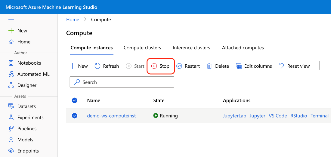
Unlike the compute clusters we used in the previous articles, compute instances don’t stop automatically after a configured period of inactivity.
Summary
Throughout the series, you’ve learned how we can use Python in several different ways to create and train models using Azure Machine Learning. This final article of the three-part series has shown how to train a TensorFlow model using Azure ML notebooks.
In this article, you’ve experienced how, with little effort, you can adapt the sample code to handle any image classification task for your own images. Most likely, you have a different number of channels (MNIST images are monochromatic) and classes. You must appropriately change the model code and the load_dataset method in such a case.
To learn everything you need to get started with Azure Machine Learning, check out Quickstart: Create workspace resources.
