Gradient Boosting with Intel’s Optimized XGBoost

The xgboost library provides scalable, portable, distributed gradient-boosting algorithms for Python*. The key features of the XGBoost algorithm are sparse awareness with automatic handling of missing data, block structure to support parallelization, and continual training. This article refers to the algorithm as XGBoost and the Python library as xgboost to distinguish between the two.

The XGBoost algorithm’s rapid rise in popularity motivated companies to develop products to support its growth. Intel has made significant contributions in this regard, introducing optimizations to every open source xgboost release starting with 0.81. The Intel^® AI Analytics Toolkit (AI Kit) includes Intel® Optimization for XGBoost* and many other optimized libraries for machine learning, such as an optimized version of Python, Scikit-learn* (sklearn), and Modin* to enhance data preprocessing and analytics.

This article focuses on the XGBoost algorithm and compares its performance to related tree-based models. We can access the XGBoost algorithm as a Python package (xgboost) using Anaconda*, Python pip, or other package managers. We install the relevant dependencies step-by-step as we progress through this tutorial.

What is Gradient Boosting?

Gradient boosting, also known as a stochastic gradient or a gradient boosting machine, combines the ideas of gradient descent and ensemble boosting to create an algorithm that reduces errors as new decision trees are added to the sequence. It minimizes errors by iteratively computing the gradient of a convex function in the direction of a minimum. In this tutorial, we train and test a boosted tree evaluated on the log loss, which is sklearn’s default loss function.

Decision tree models are particularly susceptible to underfitting, as their simple design favors interpretability. We can use ensemble learning to reduce the risk of underfitting. A single ensemble architecture combines multiple models into one architecture that uses the base learner’s predictions to train additional models until convergence. The two main types of ensembles are bagging and boosting. Bagging selects data points randomly with replacement and equal probability, thereby reducing variance. Boosting selects data points based on the performance so far, reducing bias. The XGBoost algorithm combines these concepts to ensure low bias and low variance.

How to Perform Gradient Boosting

In this project, we implement, evaluate, and compare a regular decision tree model, a gradient-boosting decision tree, and the XGBoost algorithm using Intel Optimization for XGBoost. The task is to take a set of attributes that describe a car and classify its quality as unacceptable, acceptable, good, or very good.

Let’s begin. First, download the dataset from the University of California at Irvine (UCI) machine learning repository’s website or Kaggle*.

The dataset contains the following six features used to classify a car’s quality:

• Buying price
• Maintenance cost
• Number of doors
• Number of passengers
• Luggage boot
• Estimated safety level

Second, import the necessary libraries and load the entire dataset. Run the code snippets in your Anaconda environment on your preferred integrated development environment (IDE). We run all the code in this article in a Jupyter* Notebook. Following this tutorial in a notebook will minimize the risk of errors when you run it.

import numpy as np
import pandas as pd
import matplotlib.pyplot as plt
import seaborn as sns; sns.set()
import warnings
import category_encoders as ce
from sklearn.metrics import accuracy_score
from sklearn.model_selection import train_test_split
import time
import warnings

df = pd.read_csv("pathToData\\car_evaluation.csv")

Third, we conduct some exploratory data analysis to understand the data better. The pandas package command df.info returns relevant information about the characteristics of our data frame, like the presence of null values and our features’ data types.

Execute df.info(). This is the result:

<class 'pandas.core.frame.DataFrame'>
RangeIndex: 1727 entries, 0 to 1726
Data columns (total 7 columns):
 #   Column   Non-Null Count  Dtype 
---  ------   --------------  ----- 
 0   vhigh    1727 non-null   object
 1   vhigh.1  1727 non-null   object
 2   2        1727 non-null   object
 3   2.1      1727 non-null   object
 4   small    1727 non-null   object
 5   low      1727 non-null   object
 6   unacc    1727 non-null   object
dtypes: object(7)
memory usage: 94.6+ KB

Although we can infer what each column represents based on the dataset’s description, the columns currently have generic names. So, let’s pass a list of names to give each column a descriptive label.

df.columns= ['buying','maint','doors','persons','lug_boot','safety','class']

Before instantiating our models, we need to encode all our categorical variables and split our dataset into training and testing. We can easily split our data with sklearn’s train_test_split function:

# Separate class column for target variable
X = df.drop(['class'], axis=1)
y = df['class']
 
X_train, X_test, y_train, y_test = train_test_split(X, y, test_size = 0.3, random_state = 42)

Note that the nature of the categorical variable is ordinal. We can use the ordinal encoder (OrdinalEncoder) from the categorical encoders package to encode our data in this manner:

# Encode training features with ordinal encoding
encoder = ce.OrdinalEncoder(cols=X_train.columns)

X_train = encoder.fit_transform(X_train)
X_test = encoder.transform(X_test)

In the following three sections, we implement three approaches for comparison: a simple decision tree, a gradient boosting machine, and Intel’s XGBoost algorithm.

Creating a Simple Decision Tree

The scikit-learn Python package provides many functionalities to access, train, and evaluate machine learning models. The DecisionTreeClassifier corresponds to a simple decision tree model meant for classification tasks.

Let’s establish our benchmark as the accuracy score of the default implementation of this model after training.

We run the following code in our chosen IDE to instantiate and train a decision tree classifier with sklearn.

from sklearn.tree import DecisionTreeClassifier
 
tree = DecisionTreeClassifier(random_state=42)
 
# fit the model
tree.fit(X_train, y_train)

Next, we evaluate our model’s prediction by computing the accuracy score, which is the percentage of correctly classified predictions, using the code below:

# Predict and test on test data
y_hat = tree.predict(X_test)
accuracy_score(y_test, y_hat)
> 0.9441233140655106

Therefore, our benchmark score is 94.4 percent prediction accuracy.

Gradient Boosting

We then use the GradientBoostingClassifier class to implement gradient boosting into a simple decision tree for classification, like the one we just created. To see how boosting affects the model’s performance, we run the following code:

from sklearn.ensemble import GradientBoostingClassifier

boostedTree = GradientBoostingClassifier(random_state=42)
boostedTree = boostedTree.fit(X_train, y_train)

boosted_y_hat = boostedTree.predict(X_test)
accuracy_score(y_test, boosted_y_hat)
> 0.9653179190751445

Prediction accuracy improved by approximately two percentage points from 94.4 percent to 96.5 percent. With gradient boosting, we give up speed for increased accuracy and interpretability.

To access insights about the importance of each variable, according to our model, we use the feature_importances_ function as follows:

boostedTree.feature_importances_
array([0.14527816, 0.10707345, 0.01425489, 0.36412543, 0.04581993, 0.32344813])

The method returns an array containing the corresponding weights for each of the variables in our dataset.

XGBoost

To speed up training and inference, we use Intel Optimization for XGBoost. To install it as part of the AI Kit, let’s create a new Anaconda environment.

Run the following command if you’re using the command prompt. Otherwise, use the GUI interface. For additional details, refer to the official documentation.

conda create –name envName

Then, we install the AI Kit like any other package using conda:

conda install intel-aikit-modin -c intel

Finally, before accessing the tools, we activate the environment by running Anaconda’s command prompt:

conda activate intel-aikit-modin

With Intel’s AI Kit installed and activated, we can proceed as we would with the regular xgboost framework. Since the AI Kit also includes an optimized version of Scikit-learn, we can follow the same syntax to fit and test our XGBoost algorithm. The following code instantiates XGBoost by minimizing the log loss and computing the prediction accuracy. To prevent unexpected errors, ensure you have version 1.5 or lower of xgboost. You can check your version with the following command if you're using a notebook like Jupyter or Google Colab*. If you’re interacting from the terminal, remember not to include the exclamation mark.

!xgboost --version
> XGBoost: 1.5.0

Otherwise, run the following:

import xgboost
print(xgboost.__version__)

Finally, we can load, train and test the model with just a few lines of code.

from xgboost import XGBClassifier
 
xgb = XGBClassifier(eval_metric='mlogloss')
xgb.fit(X_train, y_train)
# Predict and test on test data
xgb_y_hat = xgb.predict(X_test)
accuracy_score(y_test, xgb_y_hat)
> 0.9691714836223507

This is a somewhat negligible improvement over our previous gradient boosting classifier from 96.5 percent to 96.9 percent. As we noted earlier in this article, this is a simple dataset. Moreover, these accuracy scores are unusually high. So, let’s explore other dimensions along which to compare our models.

Model Comparison

So far, we’ve used a single train-test split to assess the accuracy score of each model. For a small dataset like ours, this increases the sensitivity to overfitting. A better approach is to train the model in batches and shuffle the data in each training iteration.

The model_selection class from sklearn provides functionality to implement K-fold cross-validation. By leveraging K-fold cross-validation, we can better capture the actual average performance of each model without risking a data leak.

from sklearn import model_selection
 
models = [('TR', tree),
          ('BT', boostedTree),
          ('XGB', xgb)]
 
# evaluate each model in turn
results = []
names = []
scoring = 'accuracy'
for name, model in models:
    time_start = time.time()
    kfold = model_selection.KFold(n_splits=10)
    cv_results = model_selection.cross_val_score
                 (model, X_train, y_train, cv=kfold, scoring=scoring)
    results.append(cv_results)
    names.append(name)
    time_end = time.time()
    msg = f"{name}: Mean score {cv_results.mean()} - 
          Std {cv_results.std()} - Seconds {round((time_end - time_start), 3)}"

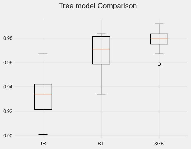
Note that your results may differ because cross-validation consists of selecting K randomly shuffled subsets of the entire dataset repeatedly. So, the scores may vary depending on the samples used for each training session. Here, we can see the XGBoost model, on average, provides a significant improvement over the boosted tree in terms of both accuracy and runtime.

> TR: Mean score 0.932961432506 - Std 0.0186055525846 - Seconds 0.043
> BT: Mean score 0.966907713498 - Std 0.0156554455448 - Seconds 3.529
> XGB: Mean score 0.97847796143 - Std 0.0099176064591 - Seconds 2.047

A boxplot helps us visually understand how performance accuracy varies among models, as shown below.

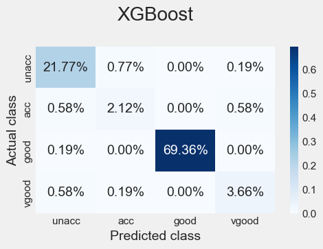
Finally, we can plot each model’s confusion matrix to better understand how it made decisions. Remember that the correct way to read these is the percentage of times the predicted class matched the actual class (and was thus correctly classified).

All three algorithms capture the essential characteristics of a good car much better than the other possible classes, with an accuracy of 68 percent or higher, followed by the characteristics of a vehicle of unacceptable quality, with an accuracy of 20 percent or higher. The remaining two classes show exceptionally low percentage scores, suggesting the need for more data in this case.

Conclusion

In this article, we explored the XGBoost algorithm by building two simple models and comparing them to Intel’s xgboost wrapper in Python. Finally, we conducted a simple evaluation to better understand the performance of each model by measuring accuracy and runtime. The results from the K-fold (K=10) cross-validation and confusion matrices demonstrated the significant improvement that Intel’s xgboost library offers in terms of classification accuracy and runtime.

With only a few lines of code and without having to learn any new syntax, Intel’s AI Kit allowed us to improve the performance of our tree-based model seamlessly. We covered the main steps to get started with this new open source product. As previously mentioned, an optimized XGBoost algorithm is just one of the many features at our disposal. The AI Kit includes advanced capabilities to preprocess data more efficiently and enhance your project’s machine-learning pipelines. The next steps include:

• Experimenting with hyperparameter tuning
• Gaining further speed improvements by adding the daal4py package
• Testing the daal4py package on a prediction task
• Testing the algorithm with much bigger datasets

You can learn more by reading the AI Kit documentation and experimenting with Intel’s code samples.