Starting today, we embark on a journey to explore the inner workings of vector databases. These databases have surged in popularity in recent years due to the growing demands of artificial intelligence. They allow us to efficiently store and query multidimensional data. In this series of articles, we will examine how vector databases differ from conventional relational databases, why it is important to promote them, and how to implement them in C#.
Introduction
Vector databases have already been discussed in previous articles, and we encourage readers to refer to those for a foundational understanding. In this series, we will delve deeper into the inner workings by uncovering the underlying data structures such as kd-trees.
The subsequent textbooks prove useful for concluding this series.
Foundations of Multidimensional and Metric Data Structures (Samet)
Introduction to Algorithms (Cormen, Leiserson, Rivest, Stein)
Algorithms (Sedgewick, Wayne)
This article was originally published here: Implementing vector databases with kd-trees in C#
What are vector databases ?
Vector databases are specialized databases designed to efficiently store and query high-dimensional vector data. Unlike traditional relational databases that are optimized for tabular data, vector databases are tailored to handle vectors as primary data types.
They provide mechanisms for storing, indexing, and querying vectors in a manner that preserves their high-dimensional structure and enables efficient similarity search and other vector-based operations. Examples of vector databases include Milvus, Faiss, and Pinecone.
OK but why do we need to store vectors at all ?
We already have relational databases and other paradigms for storing data. So why bother with these new kinds of databases ?
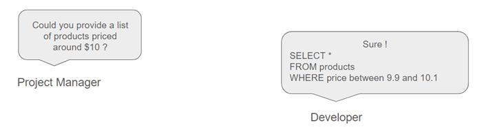
Well, conventional databases are great for storing traditional data. For instance, an e-commerce website handles transactions and products that can be represented as tabular objects with attributes, making it easy to query this data using simple SQL syntax.
However, with the advent of artificial intelligence and the need to manipulate large amounts of data, this approach becomes much less practical.

That is why a kind of preprocessing is necessary to transform data, such as documents or images, into queryable objects. This transformation, known as embedding, involves representing abstract data as vectors in traditional vector spaces.
Important
Designing this embedding is more an art than a science and depends on the specific object we want to represent (for example, documents can be modeled using the TF-IDF paradigm). Ultimately, embedding constitutes the real value added and is likely the most challenging aspect to achieve in an artificial intelligence application.
Once data is stored in a vector space, everything becomes simpler: it is easy to find similar objects by computing the similarity between two vectors, and it is easy to perform arithmetic operations on objects. For example, we can subtract one document vector from another and explore the resulting document vector.
But how to store all these vectors ?
Now that we grasp the importance of vectors, a natural question arises: how can we efficiently store and query these vectors ? We could certainly utilize existing platforms such as relational or NoSQL databases, but we will soon find that their underlying foundations are not well-suited for this purpose. Why ? Because vectors are inherently multidimensional data, and conventional databases lack native data structures capable of manipulating them.
Summary
Vector databases are databases explicitly engineered to efficiently store and query vectors (which serve as mathematical representations of abstract objects such as documents or images).
The remainder of this article aims to explore potential data structures suited for this purpose, observe them in action, and implement simplified versions to understand how they can be enhanced.
What are the applications of vector databases ?
As previously mentioned, vectors fundamentally represent multidimensional data that encapsulates abstract objects. In the following images, our embedding function is represented as f.
What are the demands associated with this data ? Put differently, what are the applications of vector databases ?
Consider a scenario where we are storing documents that describe products (for instance, on an e-commerce website) and we have defined an embedding model for representing textual data.
From this, we can develop a recommendation system: for each product in the catalog, identify the top 5 recommended products. In mathematical terms, this involves finding the 5 nearest neighbors in the vector space for each vector that represents a product in the catalog.
Important
It is evident that the embedding model is crucial and must be meticulously crafted: documents that are closest in "reality" should be close in the vector space to provide meaningful recommendations.
So, how can we conduct efficient searches ?
To make this article less abstract, let's now implement a bit of C# code to explore a very basic implementation of nearest neighbor search. This implementation will serve as a benchmark compared to the more sophisticated data structures we'll explore next.
Firstly, we will define an Embedding class to serve as a simple model for an array of doubles.
public class Embedding
{
    public double[] Records { get; set; }

    public Embedding(double[] records)
    {
        Records = records;
    }
}
Next, we will define an interface that allows us to store and query embeddings. We will begin by exploring a naive implementation of this interface, followed by a more sophisticated one.
public interface IEmbeddingStorer
{
    void LoadEmbeddings(List<Embedding> embeddings);

    List<Embedding> FindNearestNeighbours(IDistance distance, Embedding embedding, int n);
}
This interface is straightforward, containing two methods: one for loading a list of initial embeddings, and the other for finding the nearest neighbors of a target embedding.
To complete the implementation, we will also introduce an interface to represent the distance between two embeddings.
public interface IDistance
{
    double DistanceBetween(Embedding e1, Embedding e2);

    double DistanceBetween(double d1, double d2);
}
A concrete implementation could be the Euclidean distance. It's worth noting that other implementations are possible and depend on the specific application requirements.
public class EuclidianDistance : IDistance
{
    public double DistanceBetween(Embedding e1, Embedding e2)
    {
        var dimension = e1.Records.Length; var distance = 0.0;
        for (var i = 0; i < dimension; i++)
        {
            distance = distance + Math.Pow(e1.Records[i]-e2.Records[i], 2);
        }

        return distance;
    }

    public double DistanceBetween(double d1, double d2)
    {
        return Math.Pow(d1-d2, 2);
    }
}
With this groundwork laid out, we can now implement a first naive version of the FindNearestNeighbours method. This straightforward approach involves iterating over all embeddings to find the 5 nearest ones.
public class ListEmbeddingStorer : IEmbeddingStorer
{
    private List<Embedding> _embeddings;

    public void LoadEmbeddings(List<Embedding> embeddings)
    {
        _embeddings = embeddings;
    }

    public List<Embedding> FindNearestNeighbours(IDistance distance, Embedding embedding, int n)
    {
        var res = new List<EmbeddingWithDistance>();
        foreach (var e in _embeddings)
        {
            var dist = distance.DistanceBetween(e, embedding);
            if (res.Count < n) res.Add(new EmbeddingWithDistance(dist, e));
            else
            {
                var max = res.OrderByDescending(i => i.Distance).First();
                if(dist < max.Distance)
                {
                    res.Remove(max);
                    res.Add(new EmbeddingWithDistance(dist, e));
                }
            }
        }

        return res.Select(t => t.Embedding).ToList();
    }
}

public class EmbeddingWithDistance
{
    public double Distance { get; set; }

    public Embedding Embedding { get; set; }

    public EmbeddingWithDistance(double distance, Embedding embedding)
    {
        Distance = distance;
        Embedding = embedding;
    }
}
Important
Indeed, this implementation is naive because its time complexity is linear in the number of items: every record must be visited to produce the result. Therefore, it is not scalable beyond small datasets containing only several thousand items.
Modern artificial intelligence applications deal with vast amounts of data, often reaching several hundreds of millions of records. Therefore, relying on linear time search operations is not feasible and it is crucial for vector databases to efficiently find nearest neighbors, or in other words, to perform searches rapidly. Our challenge is to prioritize a data structure designed for efficient multidimensional searching.
We will now explore how to efficiently store multidimensional data by introducing the kd-tree data structure. Our goal is to effectively handle multidimensional searches.
What are binary search trees ?
In computer science, when dealing with search operations, practitioners often turn to tree structures. While we won't delve deeply into this topic here, we will draw inspiration from these data structures to implement kd-trees.
Information
Trees are extensively covered in the following authoritative textbooks.
Introduction to Algorithms (Cormen, Leiserson, Rivest, Stein)
Algorithms (Sedgewick, Wayne)
Binary search trees (BSTs) are a type of binary tree data structure that has the following properties:
- Each node in a binary search tree can have at most two children, referred to as the left child and the right child.
- All nodes in the left subtree have values less than the node's value.
- All nodes in the right subtree have values greater than the node's value.
This property ensures that the BST is ordered such that for any node, all nodes in its left subtree have values less than the node's value, and all nodes in its right subtree have values greater than the node's value.
Here's a brief example of a binary search tree.
    5
   / \
  3   8
 / \   \
2   4   10
- The root node has a value of 5.
- The left subtree of the root (with root 3) has nodes with values less than 5 (i.e., 3, 2, 4).
- The right subtree of the root (with root 8) has nodes with values greater than 5 (i.e., 8, 10).
BSTs excel in search operations, which makes them highly suitable for tasks like database indexing. It is thus natural to draw inspiration from them for our needs. But, in contrast to binary search trees which handle unidimensional data by comparing values at each node and choosing a direction, kd-trees are designed to manage multidimensional data within a tree structure. However, this requires a few fundamental changes to the approach.
What are kd-trees ?
A kd-tree is a space-partitioning data structure used to organize points in a 𝑘k-dimensional space.
-
A kd-tree is a binary tree where each node represents a point in 𝑘k-dimensional space.
-
At each level of the tree, a different dimension is used to split the space. The root node splits based on the first dimension, the next level splits based on the second dimension, and so on, cycling through the dimensions.
-
Each node in a kd-tree contains a 𝑘k-dimensional point (referred to as an embedding in our previous discussions) and references to its left and right child nodes.
Here's an example of a kd-tree structure for 2-dimensional data points (𝑘=2k=2).
level 0 (split on first dimension):
          (5, 3)
         /      \
level 1 (split on second dimension):
    (2, 4)       (9, 6)
     /   \        /   \
level 2 (split on first dimension):
(3, 1) (1, 7) (8, 5) (10, 8)
- The root node splits based on the first dimension.
- The second level splits based on the second dimension.
- The third level splits based on the first dimension again, and so on.
Information 1
In practical use cases, data points are split across more dimensions, but representing them visually becomes challenging. Therefore, illustrations of kd-trees often use 𝑘=2k=2 for simplicity.
Information 2
Kd-trees were introduced in 1975 by Jon Bentley (the original paper can be found here). While the definition we propose here differs slightly from the original in terminology, it ultimately achieves the same goal and performs efficient searches.
Information 3
A kd-tree is constructed by recursively splitting the data points based on median values of the dimensions. This ensures that the tree is balanced, which optimizes search performance.
Our definition stipulates that a kd-tree is fundamentally a binary tree. As a consequence, embeddings are inserted in a specific order: the value corresponding to the split dimension is compared to the current node's value along the same axis. If the value is greater, we recursively insert the embedding in the right node; otherwise, it is inserted in the left node. This process continues until a leaf is reached.
For example, how would we insert (4,11) into the preceding tree ? Here are the detailed steps to perform this operation.
-
The root node's first dimension is 5, and the inserted embedding's first dimension is 4, so we traverse down to the left (4<5).
-
We now compare with the node (2,4). Since we are at the second level, we compare using the second dimension. The inserted embedding's second dimension is 11, so we traverse down to the right (11>4).
-
We now compare with the node (1,7). Since we are at the third level, we compare again using the first dimension. The inserted embedding's first dimension is 4, so we traverse down to the right (1<4).
level 0 (split on first dimension):
          (5, 3)
         /      \
level 1 (split on second dimension):
    (2, 4)       (9, 6)
     /   \        /   \
level 2 (split on first dimension):
(3, 1) (1, 7) (8, 5) (10, 8)
            \
            (4, 11)
Armed with this theoretical foundation, we will now explore how to conduct efficient searches. Earlier, we discussed why finding the nearest neighbors of a specific embedding is crucial in certain applications. Our objective now is to demonstrate how this operation can be efficiently achieved using kd-trees.
The approach involves proceeding similarly to a traditional binary tree, where we traverse the entire tree to locate the subspace corresponding to the target. Unlike a classical BST however, the process does not end there, as the closest neighbors may exist in other subtrees. To illustrate our discussion, we will rely on the following example.
First case
We will start with a straightforward scenario where the embedding initially found by traversing the tree is indeed the closest neighbor: imagine that we want to find the nearest neighbor of (25,70).
Here, it is not possible for the closest point to exist in other subspaces because the distance to the boundaries (hyperplanes in mathematical terms) is greater than the distance to any point in the subtree.
Information
In mathematical terms, if the orthogonal projection along the current split axis is greater than the orthogonal projection of the target embedding along the same axis, then we can bypass every point in the subtree and move up to the parent level.
Second case
Now, let's consider a more interesting scenario: we want to find the nearest neighbor of (52,72).
The initial closest embedding found by traversing down the tree is (60,80), but it's evident that this is not the closest point to our target.
In fact, the distance to the other subtree (the one containing the point (55,1)) is less than the distance to the initially found point (60,80). Therefore, it is entirely possible that a point in this subspace could be the closest and we need to investigate it. After visiting this subspace, we continue our process towards the root and explore whether a closest embedding may exist in the left subtree of the root. In this particular case, we may end up visiting the entire tree, and thus not gain any performance compared to a naive implementation.
Very important
To conduct our searches, we begin from the most likely subspace and traverse up the tree until we reach the root. It's important to note that we must examine all levels and cannot stop prematurely. Our goal is to visit the fewest subtrees possible in the process.
Information
Searching in a kd-tree typically operates with logarithmic time complexity, which makes it highly desirable.
Now that we have a comprehensive understanding of what a kd-tree is and how it can efficiently perform searches for multidimensional data, let's put it into action by implementing it in C#. But to avoid overloading this article, readers interested in this implementation can find the continuation here.

