Excel - Displaying Your Top Row as the Column Header

Introduction

Excel does not give an easy way of changing your column headings to something other than the built-in A, B, C or 1, 2, 3 (R1C1) format.  However, if you format the entire table as a Table, then Excel has a useful trick to enable such a feature.

Enabling Customized Column Headers

1. Using Microsoft Excel 2013 or later (haven't tried earlier versions), create a table in Excel.
2. Make the first row the header row that you wish to see in the columns by giving it short meaningful names.
3. With a cell in your table selected, click on the "Format as Table" option in the HOME menu.
4. When the "Format As Table" dialog comes up, select the "My table has headers" checkbox and click the OK button.
5. Select the first row; which should be your header row.
6. Right-click on the grey row 1 header area and select hide.
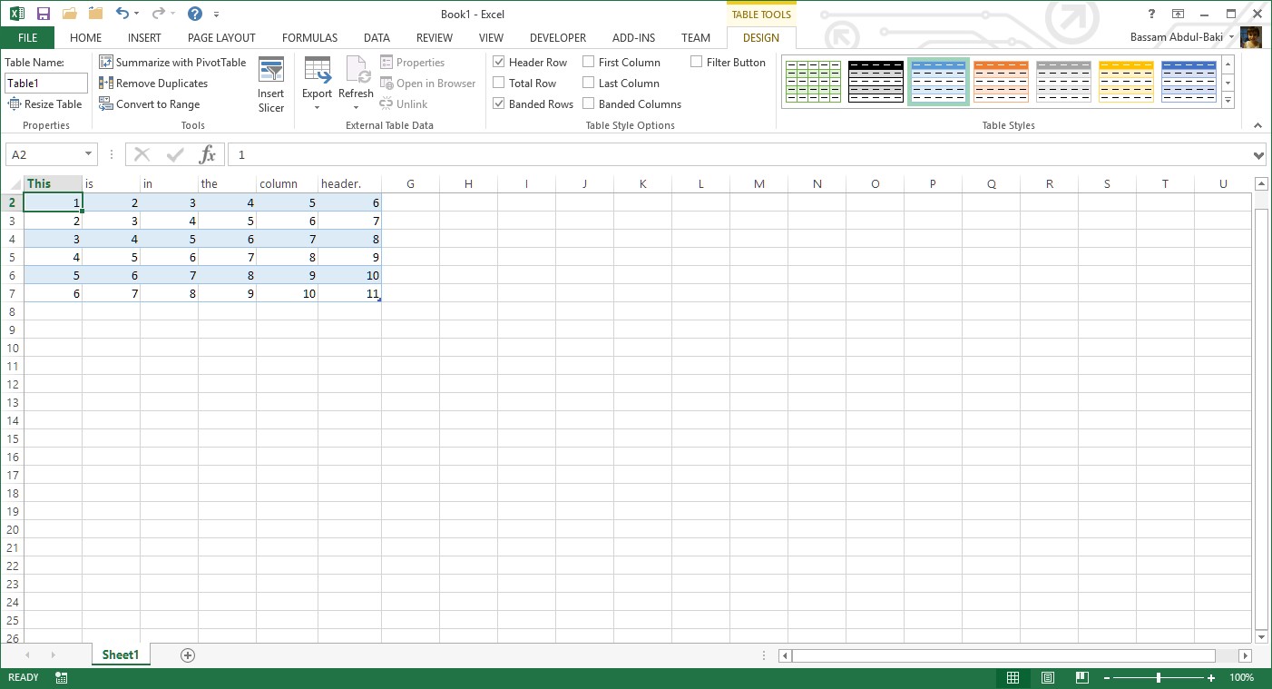
7. The column names for only the table area should now reflect the first row data.

Note: If you scroll down or right outside of the table area, the column headers switch to the built-in format.

Points of Interest

This feature did not work for row headers and only seems to work with the "Format as Table" option.

History

• 2017-05-21: Introduction