Excel 2013 Power Pivot Sorting

Introduction

While creating a Power Pivot based report, i.e., Pivot table or Pivot chart, using Month slicer is a very common requirement. There are a number of blogs that show how to sort the Month in natural order in Pivot table. You can also find some workarounds to sort Month in natural order for slicer as well. One such tip is explained well in MSDN blog here.

But with Excel 2013, there is no need to have such workarounds.

Using the Code

Assuming you have Date table with the following columns:

1. Year => 2010, 2011, 2012.......
2. Month Name => Jan, Feb, March.....
3. MonthOfYear => 1, 2, 3..... 12

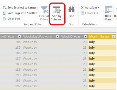
Now select the column Month Name, under sort and filter section of Home tab.

Now click on "Sort by Column.."

In this, select the Column to be sorted and sorted by. Here, sort column is MonthName and By column is MonthOfYear. Click Ok.

Now you can add the Slicer of Month Name and it will be sorted by natural order instead on alphabet.

Using this functionality, any column can be sorted by any other column within the table.