Optimizing a Function of One Variable

• Download source - 3.21 KB

Introduction

This article describes an algorithm for optimizing a function of one variable without requiring a function for the derivative. Methods that require derivatives are often fast but unstable. Methods that do not require derivatives are often stable but slow. The method implemented here, however, is stable and efficient. It was first published by Richard Brent in his book "Algorithms for Minimization Without Derivatives."

Given a function f(x) and an interval [a, b], the method finds the minimum of f(x) over [a, b]. The method can be used to maximize functions as well. To find the maximum of a function, pass in the negative of the original function. That is, the maximum of f(x) occurs at the minimum of -f(x).

Brent's method is more robust than the Newton's more familiar method. When Newton's method works, it is very fast. But when it does not work, it can go wildly wrong, producing worse answers with each iteration. Newton's method is like the girl in the nursery rhyme:

When she was good, she was very, very good.
But when she was bad she was horrid.

Brent's method is also easier to use than Newton's method because it does not require the user to supply a derivative function. The method sacrifices some efficiency for the sake of robustness, but the it is more efficient than other robust methods such as the golden section method.

Using the Code

The code given here is a single C++ function and a demo project for using it. To use the function in your own project, simply #include the header file Brent.h.

The main input to the minimization function is a templated argument, a function object implementing the objective function to minimize. The objective function must implement a public method with the signature double operator()(double x). For example, here is a class for a function object to compute the function f(x) = -x exp(-x).

class foo
{
public:
    double operator()(double x) {return -x*exp(-x);}
};

The primary reason our code requires a function object rather than simply a function is that functions that need to be optimized in applications often depend on parameters in addition to function arguments. A function object may have a dozen parameters that are fixed before finding the minimum of the resulting function of one variable.

The other arguments are the end points of the interval over which the function is minimized, the tolerance for stopping, and an output parameter for returning the location of the minimum. The return value of the minimization function is the value of the objective function at its minimum.

The signature for our minimization function is as follows.

template <class TFunction>
double Minimize
(
    TFunction& f,    // [in] objective function to minimize
    double leftEnd,  // [in] smaller value of bracketing interval
    double rightEnd, // [in] larger value of bracketing interval
    double epsilon,  // [in] stopping tolerance
    double& minLoc   // [out] location of minimum, where the minimum occurs
)

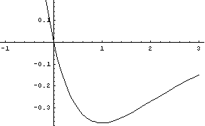
Suppose we want to find the minimum of the function -x exp(x) represented by the class foo above. Below is a plot of this function.

We find the minimum of this function twice. First we find the minimum over the interval [-1, 2] to illustrate finding a minimum in the middle of an interval. Then we find the minimum over the interval [2, 3] to illustrate the case case of the minimum occuring at one of the ends of the interval.

foo f;
double minloc; // location of the minimum
double minval; // value at the minimum

std::cout << std::setprecision(7); // display seven decimal places in output

// First minimize over [-1, 2]
minval = Minimize<foo>(f, -1, 2, 1e-6, minloc);
std::cout << "Computed minimum location: " << minloc << "\n"
          << "Exact value:               " << 1.0    << "\n"
          << "Computed minimum value:    " << minval << "\n"
          << "Exact minimum value:       " << f(1.0) << "\n\n";
          
// Now minimize over [2, 3]
minval = Minimize<foo>(f, 2, 3, 1e-6, minloc);
std::cout << "Computed minimum location: " << minloc << "\n"
          << "Exact value:               " << 2.0    << "\n"
          << "Computed minimum value:    " << minval << "\n"
          << "Exact minimum value:       " << f(2.0) << "\n\n";

In the first case, minimizing over [-1, 2], the exact minimum occurs at 1. This is the global minimum of the function. In the second case, minimizing over [2, 3], the function is increasing on this interval and so the minimum occurs at the left end point. The output shows that the results were correct to the specified tolerance of 10^-6.

Computed minimum location: 1
Exact value:               1
Computed minimum value:    -0.3678794
Exact minimum value:       -0.3678794

Computed minimum location: 2.000001
Exact value:               2
Computed minimum value:    -0.2706704
Exact minimum value:       -0.2706706

Commentary

Brent's method is an overlooked treasure from the past. It was developed decades ago (1972), and not too many people know about it now. However, the method is ideal for many applications since it is both robust and efficient. People often use the method without realizing it because it is used internally by other software packages, such as Mathematica.