Fast Numerical Integration

• Download source - 9.61 KB

Introduction

Most integrals that come up in real applications have to be evaluated numerically. Unfortunately, there is no way to write code that will efficiently and accurately evaluate any integral you throw at it. However, it is possible to write integration routines that work well on particular classes of problems.

The method presented here integrates smooth functions over finite intervals. In a sense, the method is optimally efficient, achieving the most accuracy for a given number of function evaluations.

To be more precise, the method presented here assumes that the functions being integrated are analytic. This means the functions are required to be very smooth, no discontinuities in the function or any of its derivatives. It rules out functions patched together using "if" statements, such as "return x³ if x is less than 0, and return x² if x is positive". It also rules out functions that become infinite in the middle of the integration interval. On the other hand, it does allow functions that become infinite at the ends of the integration interval.

The method presented here is the double exponential transformation. For an explanation of the mathematical details, see the article "The double-exponential transformation in numerical analysis" by Masatake Mori and Masaaki Sugihara in the Journal of Computational and Applied Mathematics, volume 127 (2001), pages 287-296. The mathematics behind the method is quite sophisticated, and will not be presented here. However, the code that implements the method is simple and easy to use.

Using the Code

The integrator is implemented in a templated class DEIntegrator. (The "DE" in the name stands for the "double exponential" algorithm at the heart of the code.) The template parameter is the class of the function to be integrated. The code uses function classes rather than function pointers because the former are more flexible. Functions often have parameters that tag along, and function classes are the way to handle that in C++. (In functional languages, you might use closures.)

To use DEIntegrator in your code, you need to add two files to your project, DEIntegrator.h and DEIntegratorConstants.h, and you need to add #include "DEIntegrator.h" in the file where you want to call the integrator.

DEIntegrator has two overloaded versions of the Integrate method. The first is the easiest to use:

static double Integrate
(
    const TFunctionObject& f,       // [in] integrand
    double a,                       // [in] left limit of integration
    double b,                       // [in] right limit of integration
    double targetAbsoluteError      // [in] desired bound on error
)

You simply pass in the function to integrate, the interval you want to integrate over, and how accurately you want the result calculated. The return value is the value of the integral.

The other overloaded version allows you to get more information after the integral is calculated.

static double Integrate
(
    const TFunctionObject& f,       // [in] integrand
    double a,                       // [in] left limit of integration
    double b,                       // [in] right limit of integration
    double targetAbsoluteError,     // [in] desired bound on error
    int& numFunctionEvaluations,    // [out] number of function evaluations used
    double& errorEstimate           // [out] estimated error in integration
)

The two additional arguments let you know how many function evaluations were required in computing the integral as well as the algorithm's estimate of the error. Note that targetAbsoluteError specifies how small you want the error to be, but errorEstimate estimates how small the error actually is. Often, the latter will be much smaller than the former, i.e., the method will do a better job than you asked for. However, if the method has difficulty with your integrand (say, due to a strong singularity at one of the end points), then errorEstimate may be larger than targetAbsoluteError, letting you know there is a problem.

Example 1

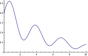
Suppose we want to integrate f(x) = exp(-x/5) (2 + sin(2x)) from 0 to 10, plotted below:

It turns out that this integral can be calculated exactly. It equals 9.1082396073230. This is a somewhat artificial example: usually, you use numerical integration for integrals that cannot be calculated exactly. But, exact integrals are useful for illustrations and testing. Suppose we want to numerically evaluate the integral to six decimal places.

First, we write our function object:

class DemoFunction
{
public:
    double operator()(double x) const
    {
        return exp(-x/5.0)*(2.0 + sin(2.0*x));
    }
};

Then, we evaluate its integral as follows:

DemoFunction f;
int evaluations;
double errorEstimate;
double integral = DEIntegrator<DemoFunction>::Integrate
        (f, 0, 10, 1e-6, evaluations, errorEstimate);
std::cout << integral << ", " << errorEstimate 
          << ", " << evaluations << "\n";

The output is:

9.10823960732284, 5.21017118337852e-009, 97

And, so in this example, we requested that the error be less than 10^-6, and the method estimates that the error was less than 5 × 10^-9, and in fact, the error was more like 10^-13. The method under-promised and over-delivered. It used 97 function evaluations in the process.

Example 2

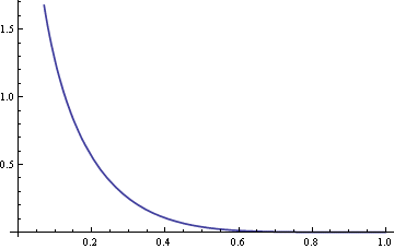
As another example, we look at f(x) = x^-1/3(1-x)⁵, plotted below. We want to integrate this function over the interval from 0 to 1. This example is to show that the integrand does not need to be analytic everywhere, just on the interior of the integration interval. In other words, it's OK if the function blows up at one or both of the ends.

We implement a function object for our integrand as follows:

class DemoFunction2
{
public:
    double operator()(double x) const
    {
        return pow(1.0 - x, 5.0)*pow(x, -1.0/3.0);
    }
};

Now, suppose we only want the estimated integral. We're not interested in counting how many function evaluations were required or the estimated error. In this case, the code to evaluate the integral is more compact.

DemoFunction2 f2;
integral = DEIntegrator<DemoFunction2>::Integrate(f2, 0, 1, 1e-6);
std::cout << integral << "\n";

In this case, the integral also happens to be one that can be evaluated exactly. In fact, the integral equals 2187/5236. The software computes the integral as 0.41768525570112. The error is approximately 2 × 10^-10.

Error Estimates

The error in elementary numerical integrations goes down like some constant power of the number of integration points. For example, the error in Simpson's rule decreases like N^-4 where N is the number of integration points. But, the error in the method presented here decreases exponentially. Specifically, the error is on the order of exp(-cN/log(N)). See this page for the mathematical details.

Internally, the code monitors its own error rate by comparing the differences in consecutive iterations to those the theory would predict. This allows the user to specify an error tolerance, and it allows the code to estimate after the fact how well it did.

Discussion

The method discussed here accurately and efficiently integrates analytic functions over a finite interval. The method is as efficient as possible for the class of functions it integrates, in a technical sense described here.

Unlike most methods presented in college courses, the method presented here does not assume that the function being integrated behaves roughly like a polynomial. Integrands may be singular at an end point, as in Example 2, without harming the accuracy of the method. Also, unlike more elementary methods, the convergence rates are exponential rather than polynomial. This means the method presented here converges very quickly.

There are variations of the double exponential rule for integrals over unbounded regions. Unfortunately, these are difficult to implement in general; the software needs to know more details about the function being integrated. A simpler approach would be to transform the integration problem into one that can be computed with the software presented here. The most obvious approach would be to truncate the unbounded integral to a bounded integral. Another approach would be to use a change of variables to transform the integral into a new integral over a bounded interval.

Truncating an integral over an unbounded region is not recommended. It can be difficult to decide where to truncate. Picking too small an interval can lead to an inaccurate answer. Picking too large an interval can lead to wasting time integrating over regions where the integrand is essentially zero.

Using a change of variables to transform the integral may be more efficient and accurate. For integrals over (0, ∞), a common change of variables is x = t/(1-t). This transforms the integral of f(x) from 0 to ∞ into the integral of f(t/(1-t)) /(1-t)² from 0 to 1. For integrals over (-∞, ∞), variables x = tan(t) transforms the integral of f(x) from -∞ to ∞ into the integral of f(tan(t)) (1 + sec²(t)) from -1 to 1. These changes of variables often work well. It is possible to get better performance by crafting a transformation specifically for your integration problem, but this is usually not necessary.

History

• 5^th December, 2008: Initial version.
• 8^th December, 2008: Added discussion of error estimates.
• 29^th June, 2009: Added discussion of integrals over unbounded regions.
• 4th May, 2015: Fixed bug in handling target absolute error.