Introduction
You may have heard about the Stanford University’s machine learning on-line course given by Prof. Andrew Ng. in 2011; it was a great course with lots of real world examples. During the course, I’ve realized that GPUs are the perfect solution for large scale machine learning problems. In fact, there are many examples about supervised and unsupervised learning all around the internet. Being a fan of both GPGPU and Machine Learning technologies, I came up with my own perspective to run machine learning algorithms with huge amount of data on the GPUs.
I already presented the solution recently at the South Florida Code Camp 2012. Everybody was interested in these two subjects a lot; therefore I decided to share it on my blog. The example in this post is neither the only solution nor the best solution. I hope it will help you one day solve your own machine learning problem.
There are a lot of concepts to machine learning but in this post, I’m only scratching the surface. If you already know about GPGPU and Machine Learning, you can just go to the source code at this link, download the Visual Studio 2010 projects and try it out.
I’ve also prepared the same example using CUBLAS with vectorized implementation of the polynomial regression algorithm, but the CUBLAS example would require more in depth explanations. Therefore, I’m posting this example first which is a simplified implementation. If you are interested in CUBLAS implementation, please let me know and I can send you that copy.
Background
Machine Learning
If you are already familiar with machine learning, you can skip the brief introduction and jump directly to the Large Scale Machine Learning section. Or if you want to learn more about machine learning, please follow the links or check out the Stanford course I’ve mentioned at the beginning.
Machine learning algorithms allow computers to recognize complex patterns. It focuses on the prediction, based on known properties learned from the training data. We are using machine learning algorithms every day dozens of times maybe unknowingly: every time we get a book or movie recommendation or every time we do a web search. In 1959, Arthur Samuel described Machine learning as: Field of study that gives computers the ability to learn without being explicitly programmed. It has been a while machine learning was first introduced, and it is gaining popularity again with the rise of Big Data.
Figure 1 shows how some of the machine learning processes work. On phase 1, given a data set, a machine learning algorithm can recognize complex patterns and come up with a model. In most cases, this phase is the bulk of the computation. In the second phase, any given data can run through the model to make a prediction. For example if you have a data set of house prices by size, you could let the machine learn from the data set and let it predict house price of any given size.
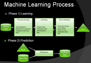
Figure 1
It does this by recognizing the function which defines the relation between the different features of the problem. A linear problem with two dimensions, like house price (the house size is the feature and the house price is the label data), can be expressed with the f(x) = ax + b model. Figure 2 shows how one feature can be used on a linear regression problem to predict new house prices. The term “hypothesis” was used in the Stanford course to describe the model.
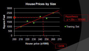
Figure 2
Depending to the data set, more complex functions can be used. In Figure 3, you can see how the complexity can grow easily from 2 dimensions linear to hundreds of dimensions polynomial. In a spam filtering problem, the different features could be words in the email or in a face recognition problem, the features could be the pixels of the image. In the house price prediction example, features are properties of the house which are affecting the price, e.g., size, room count, floors, neighborhood, crime rate, etc.
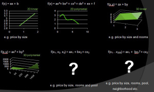
Figure 3
There are many machine learning algorithms for different problem types. The most common groups of these algorithms are Supervised Learning, Unsupervised Learning. Supervised learning is used on problems where we can provide the output values for the learning algorithm. For example: house prices for some house features is the output value, therefore house price prediction is a supervised learning problem. Data with these output values is named as “labeled data”. On the other hand, unsupervised learning does not require output values, patterns or hidden structures can be recognized just with feature data. For example: clustering social data to determine groups of people by interest would not require to define any output value, therefore it is an unsupervised learning problem.
Gradient Descent
In supervised learning problems, the machine can learn the model and come up with a hypothesis by running a hypothesis with different variables and testing if the result is close to the provided labels (calculating the error). Figure 4 shows how a training data is plot and the error is calculated. An optimization algorithm named Gradient Descent (Figure 5) can be used to find the optimum hypothesis. In this simple two dimensional problem, the algorithm would run for every different value of “a” and “b”, and would try to find the minimum total error.
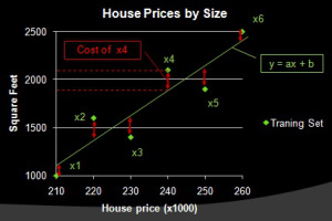
Figure 4
The pseudo code below shows how the gradient descent algorithm in Figure 5 works :
for every a and b loop until converge
errors = 0
for i = 1 to data.length
    fx = a * data[i] + b
    errors += (fx - labelData[i]) * data[i]
end for
gradient = gradient - learningRate * 1/data.length * errors
end for

Large Scale Machine Learning
Machine learning problems become computationally expensive when the complexity (dimensions and polynomial degree) increases and/or when the amount of data increases. Especially on big data sources with hundreds of millions of samples, the time to run optimization algorithms increases dramaticaly. That’s why we are looking for parallelization opportunities in the algorithms. The error summation of gradient descent algorithm is a perfect candidate for parallelization. We could split the data into multiple parts and run gradient descent on these parts in parallel. In Figure 6, you can see how the data is split into four parts and fed into four different processors. In the next step, the result is gathered together to run the rest of the algorithm.

Figure 6
Clearly, this approach would speed up the machine learning computation by almost four times. But what if we would have more cores and split the data further? That is where GPUs step into the solution. With GPUs, we can parallelize in two layers: multiple GPUs and multiple cores in every GPU. Assuming a configuration with 4 GPUs and 512 cores each, we could split down the data into 512 more pieces. Figure 7 shows this configuration along with the parallelized part on the GPU cores.
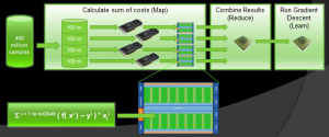
Figure 7
GPGPU
Utilizing GPUs to enable dramatic increases in computing performance of general purpose scientific and engineering computing is named GPGPU. NVIDIA is providing a parallel computing platform and programming model named CUDA to develop GPGPU software on C, C++ or Fortran which can run on any NVIDIA GPU. NVIDIA CUDA comes with many high level APIs and libraries like basic linear algebra, FFT, imaging, etc. to allow you to concentrate on the business logic rather than re-writing well known algorithms.
You can visit my previous blog posts where I’ve explained how to use NVIDIA CUDA capable GPUs to perform massively parallel computations. The examples include Monte Carlo simulation, random number generators and sorting algorithms.
House Price Prediction Example
In this post, I’ll show you how you can implement house price prediction on NVIDIA CUDA. Given a house price data set based on bedrooms, square feet and year built, it is possible to let the machine learn from this data set and provide us with a model for future predictions. Because the error calculation part of the Gradient Descent algorithm is highly parallelizable, we can offload it to the GPUs.
The machine learning algorithm in this example is Polynomial Regression, a form of the well known Linear Regression algorithm. In Polynomial Regression, the model is fit on a high order polynomial function. In our case, we will be using bedrooms, square feet, year built, square root of bedrooms, square root of square feet, square root of year built and the product of bedrooms and square feet. The reason we added the four polynomial terms to the function is because of the nature of our data. Fitting the curve correctly is the main idea behind building a model for our machine leaning problem. Logically, house prices increase by these features not in a linear or exponential way and they don’t drop after a certain peek. Therefore, the graph is more like a square root function, where house prices increase less and less compared to increasing any other feature.
Finding the right polynomial terms is very important for the success of the machine learning algorithm: having a very complex, tightly fitting function would generate too specific model and end up with overfitting, having a very simple function, like a straight line would generate too general model and end up with under fitting. Therefore, we are using additional methods like adding regularization terms to provide a better fit to your data. Figure 8 shows the gradient descent algorithm including with the regularization term lambda.

Application Architecture
The sample application consists of a C++ native DLL named LR_GPULib, for the machine learning implementation on the GPU and a C# Windows application named TestLRApp for the user interface. The DLL implements Data Normalization and Polynomial Regression using the high level parallel algorithm library Thrust on NVIDIA CUDA. I’ve mentioned on my previous blog posts about Thrust more in detail, therefore I’m not going into much detail on this post. Figure 9 shows the application architecture and also the program flow from loading the training data all the way down to making a prediction.
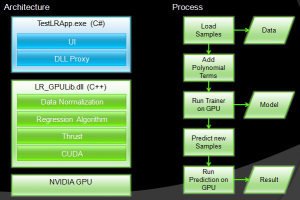
Figure 9
The application provides the UI shown below on Figure 10 to load the data, train and make a prediction with new data set. The UI also shows the hypothesis on the bottom of the dialog with all constants and features.
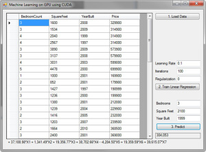
Figure 10
Implementation
The LR_GPU_Functors.cu file in the DLL contains the functors used as kernels on Thrust methods. The LR_GPU.cu file in the DLL contains the normalization, learning and prediction methods. The Learn method accepts the training data and the label data, which are all the features and all prices in two float arrays. The first thing the Learn method does is to allocate memory, add bias term and normalize the features. The reason we added the bias term is to simplify the gradient loop and the reason we normalize the features is because the data ranges are too different. E.g. square feet is four digits and bedrooms is single digit. By normalizing the features, we bring them into the same range, between zero and one. Normalization gets also executed on the GPU using the NormalizeFeatures. But the normalization requires the mean and standard deviation (std), therefore mean and std are calculated first and provided to the NormalizeFeaturesByMeanAndStd method to calculate the mean normalization.
void NormalizeFeaturesByMeanAndStd(unsigned int trainingDataCount, float * d_trainingData,
thrust::device_vector<float> dv_mean, thrust::device_vector<float> dv_std)
{
unsigned int featureCount = dv_mean.size();
float * dvp_Mean = thrust::raw_pointer_cast( &dv_mean[0] );
float * dvp_Std = thrust::raw_pointer_cast( &dv_std[0] );
FeatureNormalizationgFunctor featureNormalizationgFunctor(dvp_Mean, dvp_Std, featureCount);
thrust::device_ptr<float> dvp_trainingData(d_trainingData);
thrust::transform(thrust::counting_iterator<int>(0), thrust::counting_iterator<int>
(trainingDataCount * featureCount),
dvp_trainingData, dvp_trainingData, featureNormalizationgFunctor);
}
The Normalization code running on the GPU is implemented in the FeatureNormalizationgFunctor functor, which is simply calculating data - mean / std in parallel for every element of the data, as seen below:
...
  __host__ __device__
  float operator()(int tid, float trainingData)
  {
      int columnIdx = tid % featureCount;
      float fnorm = trainingData - meanValue[columnIdx];
      if (stdValue[columnIdx] > 0.0)
        fnorm /= stdValue[columnIdx];
      return fnorm;
  }
...
On the next step in the Learn method, the gradient descent is calculated with the for(int i = 0; i < gdIterationCount; i++) loop. As I mentioned before, the error calculation part of the gradient descent is executed in parallel but the rest is calculated sequentialy. The thrust::transform is used with the TrainFunctor to calculate f(x)-y in parallel for every sample. f(x) is simply the A*x1 + Bx2 + Cx3 + Dx4 + Ex5 + Fx6 + Gx7 + H hypothesis where x1 through x7 are the features (x1=bedrooms, x2=square feet, x3=year built, x4=square root of bedrooms, x5=square root of square feet, x6=square root of year built and x7=the product of bedrooms and square feet) and A through H are the constants which gradient descent will find out. This is shown with the Green Square on Figure 11. The TrainFunctor code snippet and the usage code snippet are shown below:

...
__host__ __device__
  float operator()(int tid, float labelData)
  {
        float h = 0;
        for (int f = 0; f < featureCount; f++)
            h += hypothesis[f] * trainingData[tid * featureCount + f];
        return h - labelData;
  }
...


...
thrust::transform(thrust::counting_iterator<int>(0),
    thrust::counting_iterator<int>(trainingDataCount),
    dv_labelData.begin(), dv_costData.begin(), tf);
...
The thrust::transform_reduce is used with the TrainFunctor2 to apply the features to the error result and sum up all of them. This is shown with the code snippet below and the Red Square on Figure 11. Rest of the Learn method calculates gradient descent part marked with Blue Square on Figure 11.
float totalCost = thrust::transform_reduce(thrust::counting_iterator<int>(0),
    thrust::counting_iterator<int>(trainingDataCount),  tf2, 0.0f, thrust::plus<float>());
Once gradient descent converges, the constants A though H of the hypothesis is returned back to the TestLRApp with the result array.
As you may guess, the prediction works by using the constants with new sample data on the hypothesis. This is done using the Predict method in the LR_GPULib library. As seen below, the Predict method normalizes the given features set and calculates the hypothesis using the constants and the normalized data with the help of the PredictFunctor. The result is the predicted house price for the given features.
...
NormalizeFeaturesByMeanAndStd(testDataCount, pdv_testData, dv_mean, dv_std);
PredictFunctor predictFunctor(pdv_testData, pdv_hypothesis, featureCount);
thrust::transform(thrust::counting_iterator(0),
thrust::counting_iterator(testDataCount), dv_result.begin(), predictFunctor);
...
struct PredictFunctor : public thrust::unary_function
{
float * testData;
float * hypothesis;
unsigned int featureCount;
PredictFunctor(float * _testData, float * _hypothesis, unsigned int _featureCount)
: testData(_testData), hypothesis(_hypothesis), featureCount(_featureCount)
{}
__host__ __device__
float operator()(int tid)
{
float sum = 0;
for(int i = 0; i < featureCount; i++)
sum += testData[tid * featureCount + i] * hypothesis[i];
return sum;
}
};
Conclusion
GPGPU, Machine Learning and Big Data are three rising fields in the IT industry. There is so much more about these fields than what I’m providing in this post. As much as I get deeper into these fields, I figure out how well they fit together. I hope this sample gave you some basic idea and maybe just one perspective how you can use NVIDIA CUDA easily on machine learning problems. As in any other software solution, this example is not the only way to do polynomial regression on house price prediction with GPUs. In fact, an enhancement would be supporting multiple GPUs and splitting down the data set into more parts.
CodeProject


