Here we’ll use the historical Bitcoin prices reorganized in sequences of 24 hours (24 prices chronologically ordered) to predict the price of the next hour.
Introduction
This series of articles will guide you through the steps necessary to develop a fully functional time series forecaster and anomaly detector application with AI. Our forecaster/detector will deal with the cryptocurrency data, specifically with Bitcoin. However, after following along with this series, you’ll be able to apply the concepts and approaches you’ve learned to any data type of a similar nature.
To fully benefit from this series, you should have some Python, Machine Learning, and Keras skills. The entire project is available in my "GitHub repository. You can also check out the fully interactive notebooks here and here.
In the previous article, we talked about anomaly detection on time series data - and now we're able to detect anomalies in past observations. But what if we want to detect them in predictions? What if we want to determine whether tomorrow’s Bitcoin price is going to be an anomaly?
Tomorrow’s Bitcoin price – and any other future data of the time series nature – can be predicted using forecasting. This approach involves fitting Machine Learning (ML) models on historical data and using them to predict future values that are not yet available.
In this project, we’ll use the historical Bitcoin prices reorganized in sequences of 24 hours (24 prices chronologically ordered) to predict the price of the next hour. To get such dataset shape, we have already defined the shift_samples function - see the previous article.
In this article, we’re going to use LSTM NN as a regressor, without the autoencoder architecture. We’ll also compare our LSTMs with Convolutional NNs in the project’s Notebook (the fully interactive one available here). Although ConvNets are out of our scope in this series, they can be useful for you in the future if LSTMs don’t work well in your scenarios.
Creating LSTM NN Regressor
Let’s create the LSTM NN regressor by issuing:
regressor = Sequential()regressor.add(layers.LSTM(256, activation='relu', return_sequences=True, input_shape=(tsteps, nfeatures),dropout=0.2))regressor.add(layers.LSTM(256, activation='relu',dropout=0.2))regressor.add(layers.Dense(1))
regressor.compile(loss='mse', optimizer='adam')
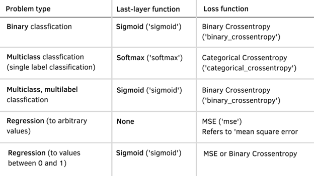
On one hand, we use MSE as a loss function because we’re trying to build a regressor and not a classifier. On the other hand, the last layer of our model doesn’t have any activation function. I’m setting only one neuron because we only have one feature in our dataset, but we’re also trying to get the next value in the given sequence. If you want to get more than one, I suggest you check this Notebook where I apply the same approach to weather data and some other variations. Use the next table to see what activation and loss functions to use depending on the task you’re trying to accomplish:

Training the Model
To train the model, issue these commands:
from tensorflow.keras.callbacks import ModelCheckpoint
checkpoint = ModelCheckpoint("/kaggle/working/regressor.hdf5", monitor='val_loss', verbose=1,save_best_only=True, mode='auto', period=1)
history2 = regressor.fit(X_train,y_train,epochs=30,batch_size=128,verbose=1,validation_data=(X_test, y_test),callbacks=[checkpoint],shuffle=False)
At the end of the process, you should get results similar to those:
Epoch 30/30
175/175 [==============================] - ETA: 0s - loss: 3.6093e-04
Epoch 00030: val_loss did not improve from 0.00024
175/175 [==============================] - 15s 87ms/step - loss: 3.6093e-04 - val_loss: 0.0023
Testing the Model
We’ve been using the ModelCheckpoint method from keras to save the best model obtained during training. Let’s use it from now on and evaluate it on the test set:
regressor = load_model("regressor.hdf5")
regressor.evaluate(X_test, y_test)
174/174 [==============================] - 1s 6ms/step - loss: 2.3974e-04
0.0002397427597315982
Not bad! When evaluating a regressor, the smaller the output, the smaller the error. The smaller the error, the better our model. In this case we’ve obtained a number very close to zero, so our rather simple model’s architecture was more than enough to get good results. However, you may face scenarios where you’ll need to design a more complex model, or invest several hours in hyperparameter tuning, and that’s totally fine. This step is more of a trial-and-error process than a "sprint" one.
Let’s see what an actual prediction looks like. To do so, let’s take the first 24 hours of the X_test dataset and invoke our regressor to predict the next hour’s value:
test = regressor.predict(X_test[0].reshape(1,24,1))
In the previous article, we scaled all our data to small values to ensure that our model could converge. Now we’re going to use the same scaler, but this time with a view to get the inverse transformation of our model’s output and obtain the actual value. Let’s see what this value is and get an idea of what the output shape is:
scaler.inverse_transform(test)
array([[6507.955]], dtype=float32)
Alright! Now we know that our model is outputting the right data shape, and that it’s up and running, ready to predict on the recent data to get future data points.
Next Step
In the next article, we’ll combine forecasting and detection on a live stream of Bitcoin price data. Stay tuned!
