Here we train our GAN to generate realistic-looking clothing images, similar to the ones found in the DeepFashion dataset.
Introduction
The availability of datasets like DeepFashion open up new possibilities for the fashion industry. In this series of articles, we’ll showcase an AI-powered deep learning system that can revolutionize the fashion design industry by helping us better understand customers’ needs.
In this project, we’ll use:
- Jupyter Notebook as the IDE
- Libraries:
- A custom subset of the DeepFashion dataset — relatively small to reduce the computational and memory overhead
We are assuming that you are familiar with the concepts of deep learning, as well as with Jupyter Notebooks and TensorFlow. If you’re new to Jupyter Notebooks, start with this tutorial. You are welcome to download the project code.
In the previous article, we designed and built a Generative Adversarial Network (GAN). In this article, we’ll train our GAN to generate realistic-looking clothing images, similar to the ones found in the DeepFashion dataset.
Training a GAN
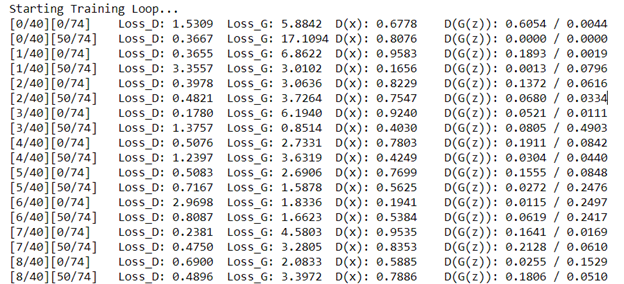
The generator training is done by reducing the loss and error between the fake and real image ((log(D(x))+log(D(G(z)). We’ll select a large number of epochs because this kind of network needs many iterations to reduce the error between the real and fake images. We’ll start with 40 epochs for training and see what results this brings. We’ll train the network on our customized dataset. Parameter and variable definitions are as follows:
- G_losses: the generator loss, calculated by summing all the losses of the generated images during the training of the generator
- D_losses: the discriminator loss, calculated by summing all the losses of real and fake batches
- D(G(z): the average discriminator outputs for all fake batches
- D(x): the average output (across the batch) of the discriminator for all real batches
img_list = []
G_losses = []
D_losses = []
iters = 0
print("Starting Training Loop...")
for epoch in range(num_epochs):
for i, data in enumerate(dataloader, 0):
netD.zero_grad()
real_cpu = data[0].to(device)
b_size = real_cpu.size(0)
label = torch.full((b_size,), real_label, dtype=torch.float, device=device)
output = netD(real_cpu).view(-1)
errD_real = criterion(output, label)
errD_real.backward()
D_x = output.mean().item()
noise = torch.randn(b_size, nz, 1, 1, device=device)
fake = netG(noise)
label.fill_(fake_label)
output = netD(fake.detach()).view(-1)
errD_fake = criterion(output, label)
errD_fake.backward()
D_G_z1 = output.mean().item()
errD = errD_real + errD_fake
optimizerD.step()
netG.zero_grad()
label.fill_(real_label)
output = netD(fake).view(-1)
errG = criterion(output, label)
errG.backward()
D_G_z2 = output.mean().item()
optimizerG.step()
if i % 50 == 0:
print('[%d/%d][%d/%d]\tLoss_D: %.4f\tLoss_G: %.4f\tD(x): %.4f\tD(G(z)): %.4f / %.4f'
% (epoch, num_epochs, i, len(dataloader),
errD.item(), errG.item(), D_x, D_G_z1, D_G_z2))
G_losses.append(errG.item())
D_losses.append(errD.item())
if (iters % 500 == 0) or ((epoch == num_epochs-1) and (i == len(dataloader)-1)):
with torch.no_grad():
fake = netG(fixed_noise).detach().cpu()
img_list.append(vutils.make_grid(fake, padding=2, normalize=True))
iters += 1

As you can see, after epoch 40, the average discriminator outputs for all fake batches
D(G(Z)) is reduced to a very attractive value. With this, the GAN is skilled enough to generate images similar to those in the dataset. If you want even better images, you need to increase the number of epochs and train again.
We can also plot a graph for the generator and discriminator loss during training.
plt.figure(figsize=(10,5))
plt.title("Generator and Discriminator Loss During Training")
plt.plot(G_losses,label="G")
plt.plot(D_losses,label="D")
plt.xlabel("iterations")
plt.ylabel("Loss")
plt.legend()
plt.show()

Visualizing Generated Images During Training
Pytorch offers a function for visualizing images generated during training as an animated video.
fig = plt.figure(figsize=(8,8))
plt.axis("off")
ims = [[plt.imshow(np.transpose(i,(1,2,0)), animated=True)] for i in img_list]
ani = animation.ArtistAnimation(fig, ims, interval=1000, repeat_delay=1000, blit=True)
HTML(ani.to_jshtml())

Generating Fashion Images from a Trained GAN
After our GAN has been trained, we can grab a batch of the fashion images it has generated by using this code.
real_batch = next(iter(dataloader))
plt.figure(figsize=(15,15))
plt.subplot(1,2,1)
plt.axis("off")
plt.title("Real Images")
plt.imshow(np.transpose(vutils.make_grid(real_batch[0].to(device)[:64], padding=5, normalize=True).cpu(),(1,2,0)))
plt.subplot(1,2,2)
plt.axis("off")
plt.title("Fake Images")
plt.imshow(np.transpose(img_list[-1],(1,2,0)))
plt.show()

Looks like our GAN was able to generate some fashion images that were similar to those found in the training dataset.
Some fast and easy ways to further improve the GAN performance are:
- Build a deeper generator using transposed convolutions or upsampling layers
- Change the type of the generator input noise to Gaussian
- Build a deeper discriminator to improve its prediction performance
- Train longer using larger number of epochs and more images
Next Steps
We’ve reached the end of our series! We achieved our goals: to create and train a deep network for fashion design category classification, and to develop a new fashion design generation using GAN.
Still, the results we achieved can be improved upon. For example, you can train your deep network on more images that contain the various clothing categories. You can also expand your project with a deep network that can detect different types of clothes in the same image using a Regional Proposed Network (RPN). Such a network would classify clothing items using a pre-trained model like the one we created in this series.
