1. Introduction
In learning of data samples when label is prior known and label of experimental data is determined based upon the learned labelled data, mathematical formulations/model which determine the new label is supervised way of learning model. When label of data samples not known in prior then one of the solution to find the label of sample data is to find various clusters (data groupings) in dataset and then labelling the cluster at later stage in the computation. This way of creating clusters for a model in order to labelling the samples (at later stage), when dataset samples labels not known in prior, is unsupervised way of learning model. One of the algorithms involved in cluster formation of unlabelled sample data is k-means algorithms.
2. Problem
How to assemble sample dataset into different clusters in such a way that each sample data (document) belongs to only one group of cluster. We are given a training set of samples {x(1),..., x(n)} or {d(1),…,d(n)} and want to group the data into a few cohesive "clusters". Here, x(i) ∈ Rd, but no labels y(i) are given. This is unsupervised learning problem. Cluster forming solution should be supported by various distance metrics.
3. Scenario
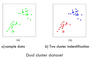
In general scenario the sample data, either geographically distributed or logically distributed, are seen exist in 'k' number of clusters. Each cluster is formed around a 'centroid/mean' and all the data samples (documents) in a particular cluster is nearer (ie. euclidean distance) to its own cluster 'mean' comparing to other cluster's mean. So each cluster has minimum variance or minimum inertia. Net inertia/variance of the complete dataset comes to its lowest.
In spatial domain one star is the mean of many spatial heavenly bodies, Sun mean cluster is labelled as Solar system. A black hole is mean star of a clusters of stars scatter around it making a galaxy. Sagittarius A is black hole mean of Milky Way galaxy. Clusters are spherical when in 3-Dimensional.

4. Notations Used and Coding Guidelines
4.1 Notations Used
Note - Word 'Centroid and Means', word 'sample data and 'document' used interchangeably.
4.2 Coding Guidelines
- Extrinsic and intrinsic identifiers are recognised. Any extrinsic identifier i.e. function parameters or names imported through "from <module> import <name> as <name>" are written as e_<identifier>.
- List variables are appended with letter 's', i.e 'document' is non sequence (list/tuple) where as 'documents' is a sequence (list/tuple).
from modulea import classa as e_classa
....
def func(e_par1, e_par2, e_samples, *e_args, *e_kwarg):
print('{(e_par1,e_par,e_samples,e_args,e_kwarg)=}')
5. Solutions
One of the mathematical computation possible to find the present 'k' clusters in the dataset is k-means algorithms. Algorithm does not change the dataset samples positions but introduces new separate centroid/mean points for each clusters. A set of 'k' new centroid/mean points.
5.1 Design
A set of 'k' random seed means/centroids from dataset are decided at the beginning (initial means). Based upon distances (i.e euclidean distance,cosine distance) to all 'k' means, each of sample data/documents are Re-Assigned to the nearest means. Each of the mean/centroid position is Re-Computed based upon mean position of all data samples/documents in its own cluster. This leads to data samples shifting its mean in re-assignment phase where as a means shifting its position (within its own cluster) in re-computation phase. Either re-assignment or re-computation does not converge leads to final cluster.
5.1.1 Algorithms Steps
- Random 'k' document points are selected as initial means.
- Each of sample data find nearest mean, computed through some mathematical distance formula (i.e. Euclidean or Cosine distances), from 'k' number of means. This is called Re-Assignment.
- Each means in 'k' means re-compute its position within its own cluster, i.e mathematical mean distance from all documents in cluster. This is called Re-Computation.
- Repeat steps 2. 3. till sample data/documents stops changing to another cluster. Stops Re-Assignments.
5.1.2 Algorithms Steps Visuals
5.1.3 Algorithms Flow Chart
Flow Chart of the algorithms can be deduced as follows.
5.1.4 Strategy Design Patterns
It follows Strategy Behavioral Design patterns
5.2 The Algorithms
k-means algorithms can be written with many possible distance measure (i.e. euclidean/cosine distances) formulations for re-assignment phase and many possible means calculation measure (i.e. mathematical means) formulation for re-computation phase.
5.2.1 Algorithms from Scratch
Python code for algorithms implementation from scratch with Euclidean distance measure and average mathematical means.
import numpy as np,random
from sklearn.metrics.pairwise import euclidean_distances,cosine_distances
def kmeans(e_samples,e_initmeans):
'''-> returns dict of labels and means'''
print(f'kmeans {e_samples[:3]=} {e_initmeans=}')
means=e_initmeans
labels=[[-1]*len(e_samples),None]
while True:
labels[1]=np.argmin(euclidean_distances(e_samples,means),axis=1).tolist()
print(f'kmeans --ReAssignment-- {labels=}')
if labels[0]==labels[1]:
return dict(labels=labels[0],means=means)
labels[0]=labels[1]
means=[np.mean([e_samples[count] for count in range(len(e_samples)) if labels[0][count]==i],axis=0).tolist() for i in range(len(e_initmeans))]
print(f'kmeans --ReComputation-- {means=}')
Function kmeans receives initial means e_initmeans as extrinsic function parameter. labels is labels[0] old label and labels[1] new label. means (Re-Computation) is calculated if Re-assignment phase brings changes to labels[1] (different from old label, labels[0]). It uses helper function get_means and matplotlib_imaging to calculate initial means and draw the matplotlib figures respectively. It returns dict of labels (as labels[0]) and means.
def get_means(*,e_samples,e_rand_state,e_k):
 print(f'get_means {e_samples[:10]=} {e_rand_state=} {e_k=}')
 return np.array(list(set(tuple(x) for x in e_samples)))[np.random.RandomState(e_rand_state).choice(len(set(tuple(x) for x in e_samples)),e_k,replace=False)].tolist()

from matplotlib import pyplot as plt
import re,os
def matplotlib_imaging(e_arg):
 color=('red','green','blue')
 fig,axes=plt.subplots()
 if e_arg:
  print(f'matplotlib_pyplot e_arg={dict({x:e_arg[x] if x!= "samples" else e_arg[x][:3] for x in e_arg})}')
  [axes.scatter(*zip(*[e_arg['samples'][count] for count in range(len(e_arg['samples'])) if e_arg['labels'][count]==i or e_arg['labels'][count]==-1]), s=10, label=str(i),c=[c] if e_arg['labels'][0]!=-1 else [[0,0,0]]) for i,c in enumerate(color[0:len(e_arg['means'])])]
  axes.scatter(*zip(*e_arg['means']), s=90, marker='*',c=color[0:len(e_arg['means'])])
  axes.legend()
  imagename="matplotlib_imaging_"+str(max([int(re.sub(r'^.*?(\d+)[.]png$',r'\1',i)) for i in os.listdir() if re.search(r'matplotlib_imaging_\d+[.]png',i,flags=re.I)] or [-1])+1)+".png"
  print(f'matplotlib_imaging saving to file {imagename}')
  fig.savefig(imagename)
get_means() function calculates initial means randomly through different RandomState initial seeding that is provided externally through e_rand_state function parameter, i.e e_rand_state=[0,None].
Running the code for rand_state=0 and rand_state=None
Input
samples=[[-14,-5],[13,13],[20,23],[-19,-11],[-9,-16],[21,27],[-49,15],[26,13],[-46,5],[-34,-1],[11,15],[-49,0],[-22,-16],[19,28],[-12,-8],[-13,-19],[-41,8],[-11,-6],[-25,-9],[-18,-3]]
print(f'--- KMEANS FROM SCRATCH ---')
print(f'{"RANDOM STATE -> 0":-^40}')
matplotlib_imaging(dict(samples=samples,**kmeans(e_samples=samples,e_initmeans=get_means(e_samples=samples,e_rand_state=0,e_k=3))))
print(f'{"RANDOM STATE -> None":-^40}')
matplotlib_imaging(dict(samples=samples,**kmeans(e_samples=samples,e_initmeans=get_means(e_samples=samples,e_rand_state=None,e_k=3))))
Output
--- KMEANS FROM SCRATCH ---
-----------RANDOM STATE -> 0------------
get_means e_samples[:10]=[[-14, -5], [13, 13], [20, 23], [-19, -11], [-9, -16], [21, 27], [-49, 15], [26, 13], [-46, 5], [-34, -1]] e_rand_state=0 e_k=3 e_init='random'
kmeans e_k=3 e_samples[:3]=[[-14, -5], [13, 13], [20, 23]] e_initmeans=[[19, 28], [-14, -5], [11, 15]]
kmeans --ReAssignment-- labels=[[-1, -1, -1, -1, -1, -1, -1, -1, -1, -1, -1, -1, -1, -1, -1, -1, -1, -1, -1, -1], [1, 2, 0, 1, 1, 0, 1, 2, 1, 1, 2, 1, 1, 0, 1, 1, 1, 1, 1, 1]]
kmeans --ReComputation-- means=[[20.0, 26.0], [-25.857142857142858, -4.714285714285714], [16.666666666666668, 13.666666666666666]]
kmeans --ReAssignment-- labels=[[1, 2, 0, 1, 1, 0, 1, 2, 1, 1, 2, 1, 1, 0, 1, 1, 1, 1, 1, 1], [1, 2, 0, 1, 1, 0, 1, 2, 1, 1, 2, 1, 1, 0, 1, 1, 1, 1, 1, 1]]
matplotlib_pyplot e_arg={'samples': [[-14, -5], [13, 13], [20, 23]], 'labels': [1, 2, 0, 1, 1, 0, 1, 2, 1, 1, 2, 1, 1, 0, 1, 1, 1, 1, 1, 1], 'means': [[20.0, 26.0], [-25.857142857142858, -4.714285714285714], [16.666666666666668, 13.666666666666666]]}
matplotlib_imaging saving to file matplotlib_imaging_0.png
----------RANDOM STATE -> None----------
get_means e_samples[:10]=[[-14, -5], [13, 13], [20, 23], [-19, -11], [-9, -16], [21, 27], [-49, 15], [26, 13], [-46, 5], [-34, -1]] e_rand_state=None e_k=3 e_init='random'
kmeans e_k=3 e_samples[:3]=[[-14, -5], [13, 13], [20, 23]] e_initmeans=[[-19, -11], [-18, -3], [-46, 5]]
kmeans --ReAssignment-- labels=[[-1, -1, -1, -1, -1, -1, -1, -1, -1, -1, -1, -1, -1, -1, -1, -1, -1, -1, -1, -1], [1, 1, 1, 0, 0, 1, 2, 1, 2, 2, 1, 2, 0, 1, 0, 0, 2, 1, 0, 1]]
kmeans --ReComputation-- means=[[-16.666666666666668, -13.166666666666666], [7.444444444444445, 11.666666666666666], [-43.8, 5.4]]
kmeans --ReAssignment-- labels=[[1, 1, 1, 0, 0, 1, 2, 1, 2, 2, 1, 2, 0, 1, 0, 0, 2, 1, 0, 1], [0, 1, 1, 0, 0, 1, 2, 1, 2, 2, 1, 2, 0, 1, 0, 0, 2, 0, 0, 0]]
kmeans --ReComputation-- means=[[-15.88888888888889, -10.333333333333334], [18.333333333333332, 19.833333333333332], [-43.8, 5.4]]
kmeans --ReAssignment-- labels=[[0, 1, 1, 0, 0, 1, 2, 1, 2, 2, 1, 2, 0, 1, 0, 0, 2, 0, 0, 0], [0, 1, 1, 0, 0, 1, 2, 1, 2, 2, 1, 2, 0, 1, 0, 0, 2, 0, 0, 0]]
matplotlib_pyplot e_arg={'samples': [[-14, -5], [13, 13], [20, 23]], 'labels': [0, 1, 1, 0, 0, 1, 2, 1, 2, 2, 1, 2, 0, 1, 0, 0, 2, 0, 0, 0], 'means': [[-15.88888888888889, -10.333333333333334], [18.333333333333332, 19.833333333333332], [-43.8, 5.4]]}
matplotlib_imaging saving to file matplotlib_imaging_1.png
When e_rand_state is 0, initial distribution of centroids not evenly spaced leading to common centroid to two clusters at [-25.857142857142858, -4.714285714285714].
5.2.2 Algorithms from sklearn.cluster package
sklearn.cluster has KMeans algorithm python function which takes primary parameters as
n_clusters - Number of clusters
init - Algorithm to calculate initial means, i.e 'random', 'kmeans++' or initial means ndarray itself.
random_state - Seeding to RandomState class object, i.e. None, or any integer
Two cases are taken. First case init argument is passed as list of initial means/centroids, whereas second case init argument is random. First case initial means is same as in '5.2.1 scratch implementation' that is initial means returned from get_means function for e_rand_state=0. So final means is also the same, i.e final 'means': [[20.0, 26.0], [-25.857142857142858, -4.714285714285714], [16.666666666666668, 13.666666666666666]]
Input
from sklearn.cluster import KMeans
samples=[[-14,-5],[13,13],[20,23],[-19,-11],[-9,-16],[21,27],[-49,15],[26,13],[-46,5],[-34,-1],[11,15],[-49,0],[-22,-16],[19,28],[-12,-8],[-13,-19],[-41,8],[-11,-6],[-25,-9],[-18,-3]]
print(f'--- KMEANS FROM SKLEARN PACKAGE ---')
kmeans_library=KMeans(n_clusters=3,init=np.array(get_means(e_samples=samples,e_rand_state=0,e_k=3))).fit(samples)
print(f'{"RANDOM STATE -> 0":-^40}')
matplotlib_imaging(dict(samples=samples,means=kmeans_library.cluster_centers_.tolist(),labels=kmeans_library.labels_.tolist()))

print(f'{"RANDOM STATE -> None":-^40}')
kmeans_library=KMeans(n_clusters=3,init='random',random_state=None).fit(samples)
matplotlib_imaging(dict(samples=samples,means=kmeans_library.cluster_centers_.tolist(),labels=kmeans_library.labels_.tolist()))
Output
--- KMEANS FROM SKLEARN PACKAGE ---
get_means e_samples[:10]=[[-14, -5], [13, 13], [20, 23], [-19, -11], [-9, -16], [21, 27], [-49, 15], [26, 13], [-46, 5], [-34, -1]] e_rand_state=0 e_k=3 e_init='random'
/usr/lib/python3/dist-packages/sklearn/cluster/_kmeans.py:1035: RuntimeWarning: Explicit initial center position passed: performing only one init in KMeans instead of n_init=10.
  self._check_params(X)
-----------RANDOM STATE -> 0------------
matplotlib_pyplot e_arg={'samples': [[-14, -5], [13, 13], [20, 23]], 'means': [[20.0, 26.0], [-25.85714285714286, -4.714285714285715], [16.66666666666667, 13.666666666666666]], 'labels': [1, 2, 0, 1, 1, 0, 1, 2, 1, 1, 2, 1, 1, 0, 1, 1, 1, 1, 1, 1]}
matplotlib_imaging saving to file matplotlib_imaging_2.png
----------RANDOM STATE -> None----------
matplotlib_pyplot e_arg={'samples': [[-14, -5], [13, 13], [20, 23]], 'means': [[-15.88888888888889, -10.333333333333334], [-43.800000000000004, 5.4], [18.33333333333333, 19.83333333333333]], 'labels': [0, 2, 2, 0, 0, 2, 1, 2, 1, 1, 2, 1, 0, 2, 0, 0, 1, 0, 0, 0]}
matplotlib_imaging saving to file matplotlib_imaging_3.png
5.2.3 Complexity of the Algorithms
I - Number of iterations
N - Number of documents, i.e. for image it is number of pixels
M - Number of components/features per sample/document, i.e. for image it is (R,G,B)
K - Number of centroids
Re-Assignment phase - Each vector operation cost O(M) for all 'M' features/components. Each of 'N' vectors does operation with each of 'K' centroids,. Total complexity sums up to O(KNM)
Re-Computation phase - Each of 'N' document vectors of ,dimension 'M', gets added to a centroid once. Total complexity sums up to O(NM)
For 'I' iterations, algorithms complexity sums up to O(IKNM)
6. External References
- k-means subsection in
https://scikit-learn.org/stable/modules/clustering.html
- Chapter 14 "DIFFERENTIATING FUNCTIONS OF SEVERAL VARIABLES" in Calculus: Single and Multi variable
https://www.wiley.com/en-us/Calculus%3A+Single+and+Multivariable%2C+7th+Edition-p-9781119320494
7. Cardinality count 'k' issues
One of the issues that we can see is initial 'k' centroid (seed) positions. This is in addition to issue of fixed number of cardinality 'k' we choose. Here we have chosen random 'k' centroids from data samples/documents with numpy random seed value. If initial centroid (seed) value changes, resultant cluster would also change and may lead to unwanted result. Think of a case when an initial centroid lies with an outlier leading to common centroid for legitimate clusters, i.e seen in the case of 'random_seed=0' in previous example under Solutions -> "The Algorithms", Section 5.2, whereas the desired means distribution should be more inclined towards bigger clusters. i.e. as seen with random_seed=None
Random state 0 - Two bigger clusters leads to same centroid
In order to have predictable result, initial kmeans distribution should be assigned as wide as possible covering each subsection in the dataset where cluster distribution size probability is larger. 'kmeans++' is the possible way to do so. It is added as an option in the 'get_means' helper function. Another parameter e_distance_metric is also added, that is distance algorithm used to calculate the distance between a dataset sample vector and a mean vector, i.e. euclidean_distance, cosine_distances
def get_means(*,e_samples,e_rand_state,e_k,e_init_type,e_distance_metric):
 print(f'get_means {e_samples[:10]=} {e_rand_state=} {e_k=} {e_init_type=}')
 if e_init_type=='random':
  return np.array(list(set(tuple(x) for x in e_samples)))[np.random.RandomState(e_rand_state).choice(len(set(tuple(x) for x in e_samples)),e_k,replace=False)].tolist()
 elif e_init_type=='kmeans++':
  samples=e_samples[:]
  means=[e_samples[0]]
  tmpvar=None
  rs=np.random.RandomState(e_rand_state)
  for i in range(0,e_k):
   tmpvar=np.min(e_distance_metric(samples,means),axis=1)
   tmpvar=rs.choice(len(samples),p=tmpvar/np.sum(tmpvar))
   means[i:i+1]=[samples[tmpvar]]
   samples[tmpvar:tmpvar+1]=[]
  return means
 else:
  raise Exception(f"{e_init_type=} can either be 'random' or 'kmeans++' ...")
8. Experimental Results
8.1 Experimental Design
8.1.1 Designing of testing setup
Experimental algorithms is designed in 'strategy' design patterns. Algorithms takes extra parameter as e_external_func and e_distance_metric and e_mean_metric.
e_external_func is polymorphic for various routines,ie. graphics imaging routines, graphics animation routines.e_distance_metric is polymorphic for distance measurement of sample data to all 'k' means (Re-Assignment phase) in order to select closest 'mean' ,i.e euclidean_distances, cosine_distances, cosine_similarity.e_mean_metric is used for 'Re-Computation' phase.
                 ---------------------
                 | 'distance_metric' |
                 ---------------------
                  ^  / \       / \ / \
                  |   -         -   -
                  |   |         |   |
                  | ----------- |   -----------------
                  | |Euclidean| |   |Cosine Distance|
                  | ----------- |   -----------------
                  |             |
                  |       ---------------------
                  |       | Cosine Similarity |
                  |       ---------------------
                  |
                  | <<'strategy design pattern'>>
                  |
                 / \
                 \ /
                  .
        ----------------------
        |  kmeans algorithms |
        ----------------------
         .              .
        / \            / \
        \ /            \ / <<'strategy design
         |              |     pattern'>>         ----------------
         |              +----------------------> | 'Mean Metric'|
         |                                       ----------------
         |<<'strategy design pattern'>>              / \     / \
         v                                            -       -
      ----------------------                          |       |
      | 'external_func'    |               ----------------  -----------
      ----------------------               | Component Mean| | ....... |
        / \             / \                ----------------- -----------
         -               -
         |               |
--------------------  ----------------------
|matplotlib_imaging|  |matplotlib_animation|
--------------------  ----------------------
In design kmeans algorithm function contains extra external_func, mean_metric and e_external_func classes (as compared to 'kmeans' function from section 5.2) which are passed to the function as parameter. Classes are polymorphic and any of the derived classes object would be passed as argument to function call.
8.1.2 Testing on "Solutions -> The Algorithms" Section 5.2 data
Setting up the test program and testing it on dataset presented in Solution -> "The Algorithms" section 5.2. 'kmeans' algorithm function is modified. matplotlib_imaging and matplotlib_animation functions are passed to e_external_func parameter whereas as per design e_distance_metric and e_mean_metric added for generic custom Re-Assignment and Re-Computation calculations.
import numpy as np
from sklearn.metrics.pairwise import euclidean_distances,cosine_distances
import types
def kmeans(e_samples,e_initmeans,e_distance_metric,e_external_func,e_mean_metric=np.mean):
'''-> returns dict of samplecluster pair and means'''
print(f'kmeans {e_samples[:3]=} {e_initmeans=}')
means=e_initmeans
e_external_func=(e_external_func if not type(e_external_func)==types.FunctionType else [e_external_func]) if e_external_func else e_external_func
labels=[[-1]*len(e_samples),None]
while True:
labels[1]=np.argmin(e_distance_metric(e_samples,means),axis=1).tolist()
print(f'kmeans --ReAssignment-- {labels[0][:20]=} {labels[1][:20]=} nonequaldocumentcount={len([count for count in range(len(e_samples)) if labels[0][count]!=labels[1][count]])}/{len(e_samples)}')
[i(dict(samples=e_samples,labels=labels[0],means=means)) for i in e_external_func] if e_external_func else None
if labels[0]==labels[1]:
[i(None) for i in e_external_func] if e_external_func else None
return dict(labels=labels[0],means=means)
labels[0]=labels[1]
means=[e_mean_metric([e_samples[count] for count in range(len(e_samples)) if labels[0][count]==i],axis=0).tolist() for i in range(len(e_initmeans))]
print(f'kmeans --ReComputation-- {means=}')
from matplotlib.patches import Rectangle
from matplotlib import animation
def matplotlib_animation(e_arg):
fig,axes=None,None
def animate(framecount):
print(f'matplotlib.animate {framecount=} {matplotlib_animation.data[framecount]=}')
nonlocal fig,axes
width,height=3,3
color=('red','green','blue')
[x.clear() for x in axes]
[x.set_aspect('equal') for x in axes]
[x.set_xlim(min(list(zip(*matplotlib_animation.data[0]['samples']))[0])-10,max(list(zip(*matplotlib_animation.data[0]['samples']))[0])+10) for x in axes]
[x.set_ylim(min(list(zip(*matplotlib_animation.data[0]['samples']))[1])-10,max(list(zip(*matplotlib_animation.data[0]['samples']))[1])+10) for x in axes]
axes[0].set_title(f'Sample ReAssignment (framecount {framecount})')
axes[1].set_title(f'Mean ReComputation (framecount {framecount})')
for i,c in enumerate(color[0:len(matplotlib_animation.data[framecount]['means'])]):
axes[0].scatter(*zip(*[matplotlib_animation.data[framecount]['samples'][count] for count in range(len(matplotlib_animation.data[framecount]['samples'])) if matplotlib_animation.data[framecount]['labels'][count]==i or matplotlib_animation.data[framecount]['labels'][count]==-1]), s=10, label=str(i),c=[c] if matplotlib_animation.data[framecount]['labels'][0]!=-1 else [[0,0,0]])
axes[0].scatter(*matplotlib_animation.data[framecount]['means'][i], s=90, marker='*',c=[c])
[axes[0].add_patch(Rectangle(xy=(x[0]-width/2,x[1]-height/2),width=width,height=height,linewidth=1,color='black',fill=False)) for count,x in enumerate(matplotlib_animation.data[framecount]['samples']) if not matplotlib_animation.data[framecount]['labels'][count]<0 and not matplotlib_animation.data[framecount]['labels'][count]==matplotlib_animation.data[framecount-1]['labels'][count]]
axes[1].scatter(*zip(*[matplotlib_animation.data[framecount]['samples'][count] for count in range(len(matplotlib_animation.data[framecount]['samples'])) if matplotlib_animation.data[framecount]['labels'][count]==i or matplotlib_animation.data[framecount]['labels'][count]==-1]), s=10, label=str(i),c=[c] if matplotlib_animation.data[framecount]['labels'][0]!=-1 else [[0,0,0]])
axes[1].scatter(*matplotlib_animation.data[framecount]['means'][i], s=90, marker='*',c=[c])
[axes[1].add_patch(Rectangle(xy=(x[0]-width/2,x[1]-height/2),width=width,height=height,linewidth=1,color='black',fill=False)) for count,x in enumerate(matplotlib_animation.data[framecount]['means']) if not matplotlib_animation.data[framecount]['means'][count]==matplotlib_animation.data[framecount-1]['means'][count]]
[x.legend() for x in axes]
print(f'matplotlib_animation saving to -> matplotlib_animation_{framecount}.png')
fig.savefig(f'matplotlib_animation_{framecount}.png')
if not hasattr(matplotlib_animation,'data'):
setattr(matplotlib_animation,'data',[])
if e_arg:
matplotlib_animation.data.append(e_arg)
else:
fig,axes=plt.subplots(1,2)
fig.set_size_inches(12.80,7.20)
anim=animation.FuncAnimation(fig,animate,frames=len(matplotlib_animation.data),init_func=lambda:None,blit=False,repeat=False)
print('matplotlib_animation saving to matplotlib_animation.mp4 ...')
anim.save('matplotlib_animation.mp4',fps=1/5,extra_args=['-vcodec','libx265','-pix_fmt','yuv420p'])
import os
print('matplotlib_animation saving to matplotlib_animation.gif ...')
os.system('''ffmpeg -i matplotlib_animation.mp4 -vf "fps=1/5,scale=1280:-1:flags=lanczos,split[s0][s1];[s0]palettegen[p];[s1][p]paletteuse" -loop 0 matplotlib_animation.gif''')
setattr(matplotlib_animation,'data',[])
Test Input
samples=[[-14,-5],[13,13],[20,23],[-19,-11],[-9,-16],[21,27],[-49,15],[26,13],[-46,5],[-34,-1],[11,15],[-49,0],[-22,-16],[19,28],[-12,-8],[-13,-19],[-41,8],[-11,-6],[-25,-9],[-18,-3]]
print(f'--- EXPERIMENTAL RESULT ----')
print(f'{"RANDOM STATE -> None":-^40}')
kmeans(e_samples=samples,e_initmeans=get_means(e_samples=samples,e_rand_state=None,e_k=3,e_init_type='random',e_distance_metric=None),e_distance_metric=euclidean_distances,e_external_func=[matplotlib_imaging,matplotlib_animation])
Test Output
--- EXPERIMENTAL RESULT ----
----------RANDOM STATE -> None----------
get_means e_samples[:10]=[[-14, -5], [13, 13], [20, 23], [-19, -11], [-9, -16], [21, 27], [-49, 15], [26, 13], [-46, 5], [-34, -1]] e_rand_state=None e_k=3 e_init='random'
kmeans e_k=3 e_samples[:3]=[[-14, -5], [13, 13], [20, 23]] e_initmeans=[[-13, -19], [-25, -9], [-19, -11]]
kmeans --ReAssignment-- labels[0][:20]=[-1, -1, -1, -1, -1, -1, -1, -1, -1, -1, -1, -1, -1, -1, -1, -1, -1, -1, -1, -1] labels[1][:20]=[2, 2, 2, 2, 0, 2, 1, 0, 1, 1, 2, 1, 2, 2, 2, 0, 1, 2, 1, 2]
matplotlib_pyplot e_arg={'samples': [[-14, -5], [13, 13], [20, 23]], 'labels': [-1, -1, -1, -1, -1, -1, -1, -1, -1, -1, -1, -1, -1, -1, -1, -1, -1, -1, -1, -1], 'means': [[-13, -19], [-25, -9], [-19, -11]]}
matplotlib_imaging saving to file matplotlib_imaging_4.png
kmeans --ReComputation-- means=[[1.3333333333333333, -7.333333333333333], [-40.666666666666664, 3.0], [-1.0909090909090908, 5.181818181818182]]
kmeans --ReAssignment-- labels[0][:20]=[2, 2, 2, 2, 0, 2, 1, 0, 1, 1, 2, 1, 2, 2, 2, 0, 1, 2, 1, 2] labels[1][:20]=[0, 2, 2, 0, 0, 2, 1, 2, 1, 1, 2, 1, 0, 2, 0, 0, 1, 0, 1, 2]
matplotlib_pyplot e_arg={'samples': [[-14, -5], [13, 13], [20, 23]], 'labels': [2, 2, 2, 2, 0, 2, 1, 0, 1, 1, 2, 1, 2, 2, 2, 0, 1, 2, 1, 2], 'means': [[1.3333333333333333, -7.333333333333333], [-40.666666666666664, 3.0], [-1.0909090909090908, 5.181818181818182]]}
matplotlib_imaging saving to file matplotlib_imaging_5.png
kmeans --ReComputation-- means=[[-14.285714285714286, -11.571428571428571], [-40.666666666666664, 3.0], [13.142857142857142, 16.571428571428573]]
kmeans --ReAssignment-- labels[0][:20]=[0, 2, 2, 0, 0, 2, 1, 2, 1, 1, 2, 1, 0, 2, 0, 0, 1, 0, 1, 2] labels[1][:20]=[0, 2, 2, 0, 0, 2, 1, 2, 1, 1, 2, 1, 0, 2, 0, 0, 1, 0, 0, 0]
matplotlib_pyplot e_arg={'samples': [[-14, -5], [13, 13], [20, 23]], 'labels': [0, 2, 2, 0, 0, 2, 1, 2, 1, 1, 2, 1, 0, 2, 0, 0, 1, 0, 1, 2], 'means': [[-14.285714285714286, -11.571428571428571], [-40.666666666666664, 3.0], [13.142857142857142, 16.571428571428573]]}
matplotlib_imaging saving to file matplotlib_imaging_6.png
kmeans --ReComputation-- means=[[-15.88888888888889, -10.333333333333334], [-43.8, 5.4], [18.333333333333332, 19.833333333333332]]
kmeans --ReAssignment-- labels[0][:20]=[0, 2, 2, 0, 0, 2, 1, 2, 1, 1, 2, 1, 0, 2, 0, 0, 1, 0, 0, 0] labels[1][:20]=[0, 2, 2, 0, 0, 2, 1, 2, 1, 1, 2, 1, 0, 2, 0, 0, 1, 0, 0, 0]
matplotlib_pyplot e_arg={'samples': [[-14, -5], [13, 13], [20, 23]], 'labels': [0, 2, 2, 0, 0, 2, 1, 2, 1, 1, 2, 1, 0, 2, 0, 0, 1, 0, 0, 0], 'means': [[-15.88888888888889, -10.333333333333334], [-43.8, 5.4], [18.333333333333332, 19.833333333333332]]}
matplotlib_imaging saving to file matplotlib_imaging_7.png
matplotlib_animation saving to matplotlib_animation.mp4 ...
matplotlib.animate framecount=0 matplotlib_animation.data[framecount]={'samples': [[-14, -5], [13, 13], [20, 23], [-19, -11], [-9, -16], [21, 27], [-49, 15], [26, 13], [-46, 5], [-34, -1], [11, 15], [-49, 0], [-22, -16], [19, 28], [-12, -8], [-13, -19], [-41, 8], [-11, -6], [-25, -9], [-18, -3]], 'labels': [-1, -1, -1, -1, -1, -1, -1, -1, -1, -1, -1, -1, -1, -1, -1, -1, -1, -1, -1, -1], 'means': [[-13, -19], [-25, -9], [-19, -11]]}
matplotlib_animation saving to -> matplotlib_animation_0.png
matplotlib.animate framecount=1 matplotlib_animation.data[framecount]={'samples': [[-14, -5], [13, 13], [20, 23], [-19, -11], [-9, -16], [21, 27], [-49, 15], [26, 13], [-46, 5], [-34, -1], [11, 15], [-49, 0], [-22, -16], [19, 28], [-12, -8], [-13, -19], [-41, 8], [-11, -6], [-25, -9], [-18, -3]], 'labels': [2, 2, 2, 2, 0, 2, 1, 0, 1, 1, 2, 1, 2, 2, 2, 0, 1, 2, 1, 2], 'means': [[1.3333333333333333, -7.333333333333333], [-40.666666666666664, 3.0], [-1.0909090909090908, 5.181818181818182]]}
matplotlib_animation saving to -> matplotlib_animation_1.png
matplotlib.animate framecount=2 matplotlib_animation.data[framecount]={'samples': [[-14, -5], [13, 13], [20, 23], [-19, -11], [-9, -16], [21, 27], [-49, 15], [26, 13], [-46, 5], [-34, -1], [11, 15], [-49, 0], [-22, -16], [19, 28], [-12, -8], [-13, -19], [-41, 8], [-11, -6], [-25, -9], [-18, -3]], 'labels': [0, 2, 2, 0, 0, 2, 1, 2, 1, 1, 2, 1, 0, 2, 0, 0, 1, 0, 1, 2], 'means': [[-14.285714285714286, -11.571428571428571], [-40.666666666666664, 3.0], [13.142857142857142, 16.571428571428573]]}
matplotlib_animation saving to -> matplotlib_animation_2.png
matplotlib.animate framecount=3 matplotlib_animation.data[framecount]={'samples': [[-14, -5], [13, 13], [20, 23], [-19, -11], [-9, -16], [21, 27], [-49, 15], [26, 13], [-46, 5], [-34, -1], [11, 15], [-49, 0], [-22, -16], [19, 28], [-12, -8], [-13, -19], [-41, 8], [-11, -6], [-25, -9], [-18, -3]], 'labels': [0, 2, 2, 0, 0, 2, 1, 2, 1, 1, 2, 1, 0, 2, 0, 0, 1, 0, 0, 0], 'means': [[-15.88888888888889, -10.333333333333334], [-43.8, 5.4], [18.333333333333332, 19.833333333333332]]}
matplotlib_animation saving to -> matplotlib_animation_3.png
matplotlib_animation saving to matplotlib_animation.gif ...
8.2 Experimental Workout
8.2.1 Euclidean distance for color intensity (brightness/lightness)
Idea is to segregate pixels in an image with similar brightness values. Brightness difference between two pixels calculated through Euclidean distance. Refer to Section "10. Note on Distance Merices -> 10.1 Euclidean distance"
As can be been seen through section 9 "How it works?" Re-Assignment phase computes 'dataset RSS' as sum of each cluster RSS where each cluster RSS is sum of each cluster document euclidean distance to cluster means/centroid.
In the following image each color is taken as point in euclidean space and three clusters are formed based upon three separate color found on the image. Bold and light weighted color text are further segregated.
Two cases have been attempted, each with random seed 0, initial centroid is initialized with 'random' e_init_type in get_means function and initial centroid initialized with 'kmeans++' e_init_type in get_means algorithms function.
- Initial centroid is initialized with 'random'
e_init_type in get_means algorithms function.
import skimage.io
print(f'--- EXPERIMENTAL RESULT EUCLIDEAN DISTANCE ---')
img=skimage.io.imread('k-meansimage/testeuclidean.png')[:,:,:3]
k,distance_metric=3,euclidean_distances
print(f'experimental result Euclidean Distance {img.shape=}')
means=kmeans(e_samples=img.reshape(-1,3).tolist(),e_initmeans=get_means(e_samples=img.reshape(-1,3).tolist(),e_rand_state=0,e_k=k,e_init_type='random',e_distance_metric=distance_metric),e_distance_metric=distance_metric,e_external_func=None)
blankpageindex=set.intersection(*[set(np.argmin(distance_metric(img[row],means['means']),axis=1).tolist()) for row in range(img.shape[0])]).pop()
print(f'experimental result Euclidean Distance {means["means"]=} {blankpageindex=}')
imagebuffer=[];top=None
for row in range(img.shape[0]):
textindex=[x for x in means['labels'][row*img.shape[1]:row*img.shape[1]+img.shape[1]] if x!=blankpageindex]
if textindex:
if not top:
top=row
imagebuffer.append(dict(position=[top],index=textindex))
else:
imagebuffer[-1]['index'].extend(textindex)
gif animation for convergence , diff in reassignment(left) and recomputation(right) highlighted in rectangle else:
if top:
imagebuffer[-1]['position'].append(row)
imagebuffer[-1]['index']=max(imagebuffer[-1]['index'],key=imagebuffer[-1]['index'].count)
top=None
print(f'{imagebuffer=}')
for i in [i for i in range(k) if i!=blankpageindex]:
top=0;abc=[]
for j in range(len(imagebuffer)):
if imagebuffer[j]['index']==i:
abc.extend([np.full((imagebuffer[j]['position'][0]-top,img.shape[1],3),means['means'][blankpageindex],dtype=img.dtype),img[imagebuffer[j]['position'][0]:imagebuffer[j]['position'][1],0:img.shape[1]]])
top=imagebuffer[j]['position'][1]
skimage.io.imsave(f'image_euclidean_{i}.png',np.concatenate(abc))
print(f'saved image_euclidean_{i}.png ...')
Output
--- EXPERIMENTAL RESULT EUCLIDEAN DISTANCE ---
experimental result Euclidean Distance img.shape=(764, 733, 3)
get_means e_samples[:10]=[[193, 239, 237], [193, 239, 237], [193, 239, 237], [193, 239, 237], [193, 239, 237], [193, 239, 237], [193, 239, 237], [193, 239, 237], [193, 239, 237], [193, 239, 237]] e_rand_state=0 e_k=3 e_init='random'
kmeans e_k=3 e_samples[:3]=[[193, 239, 237], [193, 239, 237], [193, 239, 237]] e_initmeans=[[131, 162, 161], [57, 70, 70], [174, 213, 212]]
kmeans --ReAssignment-- labels[0][:20]=[-1, -1, -1, -1, -1, -1, -1, -1, -1, -1, -1, -1, -1, -1, -1, -1, -1, -1, -1, -1] labels[1][:20]=[2, 2, 2, 2, 2, 2, 2, 2, 2, 2, 2, 2, 2, 2, 2, 2, 2, 2, 2, 2]
kmeans --ReComputation-- means=[[127.80766279605095, 151.45971660954524, 150.41904956775284], [52.72048431837049, 55.89604972767216, 55.77452469173298], [192.4449186884258, 238.25252609586335, 236.26337578450497]]
kmeans --ReAssignment-- labels[0][:20]=[2, 2, 2, 2, 2, 2, 2, 2, 2, 2, 2, 2, 2, 2, 2, 2, 2, 2, 2, 2] labels[1][:20]=[2, 2, 2, 2, 2, 2, 2, 2, 2, 2, 2, 2, 2, 2, 2, 2, 2, 2, 2, 2]
kmeans --ReComputation-- means=[[124.92168134377039, 147.51023320287018, 146.51537018917156], [49.29689785403978, 51.74235378872225, 51.65610059597878], [192.5448775417265, 238.38747582590156, 236.39674928575366]]
kmeans --ReAssignment-- labels[0][:20]=[2, 2, 2, 2, 2, 2, 2, 2, 2, 2, 2, 2, 2, 2, 2, 2, 2, 2, 2, 2] labels[1][:20]=[2, 2, 2, 2, 2, 2, 2, 2, 2, 2, 2, 2, 2, 2, 2, 2, 2, 2, 2, 2]
kmeans --ReComputation-- means=[[122.69178565824572, 144.63741565981485, 143.64612427428213], [48.16435741393636, 50.31865442051605, 50.25707933798927], [192.52381992248806, 238.35906520350457, 236.36891032247664]]
kmeans --ReAssignment-- labels[0][:20]=[2, 2, 2, 2, 2, 2, 2, 2, 2, 2, 2, 2, 2, 2, 2, 2, 2, 2, 2, 2] labels[1][:20]=[2, 2, 2, 2, 2, 2, 2, 2, 2, 2, 2, 2, 2, 2, 2, 2, 2, 2, 2, 2]
kmeans --ReComputation-- means=[[121.66821256038648, 143.28973913043478, 142.30979710144928], [47.65973706955375, 49.703316198880955, 49.647386616931264], [192.51128075712353, 238.3418827307205, 236.35206489163986]]
kmeans --ReAssignment-- labels[0][:20]=[2, 2, 2, 2, 2, 2, 2, 2, 2, 2, 2, 2, 2, 2, 2, 2, 2, 2, 2, 2] labels[1][:20]=[2, 2, 2, 2, 2, 2, 2, 2, 2, 2, 2, 2, 2, 2, 2, 2, 2, 2, 2, 2]
kmeans --ReComputation-- means=[[120.29729729729729, 141.38987523087943, 140.4418183874251], [46.856427030412696, 48.78054608300276, 48.72350198343656], [192.49680449287894, 238.3221079335041, 236.33270388436628]]
kmeans --ReAssignment-- labels[0][:20]=[2, 2, 2, 2, 2, 2, 2, 2, 2, 2, 2, 2, 2, 2, 2, 2, 2, 2, 2, 2] labels[1][:20]=[2, 2, 2, 2, 2, 2, 2, 2, 2, 2, 2, 2, 2, 2, 2, 2, 2, 2, 2, 2]
kmeans --ReComputation-- means=[[119.09535833642778, 139.7466765688823, 138.82974378017082], [46.231396390027804, 48.055799048023, 47.997855695367356], [192.47726253658456, 238.29576434237453, 236.3065134802423]]
kmeans --ReAssignment-- labels[0][:20]=[2, 2, 2, 2, 2, 2, 2, 2, 2, 2, 2, 2, 2, 2, 2, 2, 2, 2, 2, 2] labels[1][:20]=[2, 2, 2, 2, 2, 2, 2, 2, 2, 2, 2, 2, 2, 2, 2, 2, 2, 2, 2, 2]
kmeans --ReComputation-- means=[[118.80967503692762, 139.35993353028064, 138.44826440177252], [46.06144233272585, 47.85384961302691, 47.796407185628745], [192.47436114298293, 238.29212258065832, 236.30294631338893]]
kmeans --ReAssignment-- labels[0][:20]=[2, 2, 2, 2, 2, 2, 2, 2, 2, 2, 2, 2, 2, 2, 2, 2, 2, 2, 2, 2] labels[1][:20]=[2, 2, 2, 2, 2, 2, 2, 2, 2, 2, 2, 2, 2, 2, 2, 2, 2, 2, 2, 2]
kmeans --ReComputation-- means=[[118.38603174603175, 138.79447245564893, 137.89520074696546], [46.06144233272585, 47.85384961302691, 47.796407185628745], [192.4517033072226, 238.26150236462954, 236.2723193736685]]
kmeans --ReAssignment-- labels[0][:20]=[2, 2, 2, 2, 2, 2, 2, 2, 2, 2, 2, 2, 2, 2, 2, 2, 2, 2, 2, 2] labels[1][:20]=[2, 2, 2, 2, 2, 2, 2, 2, 2, 2, 2, 2, 2, 2, 2, 2, 2, 2, 2, 2]
kmeans --ReComputation-- means=[[118.09259533506109, 138.38881895594224, 137.49700111069973], [45.84555883472963, 47.60598343488195, 47.54845773038842], [192.4517033072226, 238.26150236462954, 236.2723193736685]]
kmeans --ReAssignment-- labels[0][:20]=[2, 2, 2, 2, 2, 2, 2, 2, 2, 2, 2, 2, 2, 2, 2, 2, 2, 2, 2, 2] labels[1][:20]=[2, 2, 2, 2, 2, 2, 2, 2, 2, 2, 2, 2, 2, 2, 2, 2, 2, 2, 2, 2]
kmeans --ReComputation-- means=[[118.07319874050751, 138.36069642526394, 137.46893869235043], [45.84555883472963, 47.60598343488195, 47.54845773038842], [192.45049806415872, 238.2599974338138, 236.27084466223084]]
kmeans --ReAssignment-- labels[0][:20]=[2, 2, 2, 2, 2, 2, 2, 2, 2, 2, 2, 2, 2, 2, 2, 2, 2, 2, 2, 2] labels[1][:20]=[2, 2, 2, 2, 2, 2, 2, 2, 2, 2, 2, 2, 2, 2, 2, 2, 2, 2, 2, 2]
experimental result Euclidean Distance means["means"]=[[118.07319874050751, 138.36069642526394, 137.46893869235043], [45.84555883472963, 47.60598343488195, 47.54845773038842], [192.45049806415872, 238.2599974338138, 236.27084466223084]] blankpageindex=2
imagebuffer=[{'position': [13, 29], 'index': 1}, {'position': [45, 63], 'index': 1}, {'position': [68, 86], 'index': 1}, {'position': [91, 109], 'index': 1}, {'position': [112, 133], 'index': 1}, {'position': [137, 151], 'index': 1}, {'position': [186, 202], 'index': 1}, {'position': [222, 240], 'index': 0}, {'position': [245, 263], 'index': 1}, {'position': [281, 297], 'index': 1}, {'position': [320, 338], 'index': 1}, {'position': [343, 361], 'index': 1}, {'position': [366, 384], 'index': 1}, {'position': [389, 407], 'index': 1}, {'position': [412, 430], 'index': 1}, {'position': [445, 461], 'index': 1}, {'position': [479, 497], 'index': 1}, {'position': [502, 520], 'index': 1}, {'position': [525, 543], 'index': 1}, {'position': [548, 566], 'index': 1}, {'position': [591, 607], 'index': 1}, {'position': [630, 648], 'index': 1}, {'position': [653, 671], 'index': 1}, {'position': [676, 694], 'index': 1}, {'position': [699, 717], 'index': 1}, {'position': [722, 740], 'index': 1}]
/home/pi/backupbullseye_02feb/tmp/k-means.py:184: UserWarning: image_euclidean_0.png is a low contrast image
  skimage.io.imsave(f'image_euclidean_{i}.png',np.concatenate(abc))
saved image_euclidean_0.png ...
saved image_euclidean_1.png ...
Initial means allocated to [[131, 162, 161], [57, 70, 70], [174, 213, 212]], where as it is adjusted to [[118, 138, 137], [45, 47, 47], [192, 238, 236]] after re-computation.
- Initial centroid is initialized with 'kmeans++' algorithms through
get_means function.
Line
means=kmeans(e_samples=img.reshape(-1,3).tolist(),e_initmeans=get_means(e_samples=img.reshape(-1,3).tolist(),e_rand_state=0,e_k=k,e_init_type='random',e_distance_metric=distance_metric),e_distance_metric=distance_metric,e_external_func=None)
Modified to
means=kmeans(e_samples=img.reshape(-1,3).tolist(),e_initmeans=get_means(e_samples=img.reshape(-1,3).tolist(),e_rand_state=0,e_k=k,e_init_type='kmeans++',e_distance_metric=distance_metric),e_distance_metric=distance_metric,e_external_func=None)
Output
--- EXPERIMENTAL RESULT EUCLIDEAN DISTANCE ---
experimental result Euclidean Distance img.shape=(764, 733, 3)
get_means e_samples[:10]=[[193, 239, 237], [193, 239, 237], [193, 239, 237], [193, 239, 237], [193, 239, 237], [193, 239, 237], [193, 239, 237], [193, 239, 237], [193, 239, 237], [193, 239, 237]] e_rand_state=0 e_k=3 e_init='kmeans++'
kmeans e_k=3 e_samples[:3]=[[193, 239, 237], [193, 239, 237], [193, 239, 237]] e_initmeans=[[90, 99, 98], [193, 239, 237], [0, 0, 0]]
kmeans --ReAssignment-- labels[0][:20]=[-1, -1, -1, -1, -1, -1, -1, -1, -1, -1, -1, -1, -1, -1, -1, -1, -1, -1, -1, -1] labels[1][:20]=[1, 1, 1, 1, 1, 1, 1, 1, 1, 1, 1, 1, 1, 1, 1, 1, 1, 1, 1, 1]
kmeans --ReComputation-- means=[[86.30633998069459, 95.1827442443162, 94.79994249450617], [191.92494917983294, 237.55413706350004, 235.5732897252692], [3.2317738926128117, 3.9970285398382974, 3.9733259622693664]]
kmeans --ReAssignment-- labels[0][:20]=[1, 1, 1, 1, 1, 1, 1, 1, 1, 1, 1, 1, 1, 1, 1, 1, 1, 1, 1, 1] labels[1][:20]=[1, 1, 1, 1, 1, 1, 1, 1, 1, 1, 1, 1, 1, 1, 1, 1, 1, 1, 1, 1]
kmeans --ReComputation-- means=[[85.89094935529938, 94.6225966016102, 94.2506571186125], [191.88587035219538, 237.50148021817128, 235.52077936704583], [3.2317738926128117, 3.9970285398382974, 3.9733259622693664]]
kmeans --ReAssignment-- labels[0][:20]=[1, 1, 1, 1, 1, 1, 1, 1, 1, 1, 1, 1, 1, 1, 1, 1, 1, 1, 1, 1] labels[1][:20]=[1, 1, 1, 1, 1, 1, 1, 1, 1, 1, 1, 1, 1, 1, 1, 1, 1, 1, 1, 1]
kmeans --ReComputation-- means=[[85.83759090061533, 94.54782770837218, 94.17695319783704], [191.88039189662038, 237.49437131239517, 235.5137288496885], [3.2317738926128117, 3.9970285398382974, 3.9733259622693664]]
kmeans --ReAssignment-- labels[0][:20]=[1, 1, 1, 1, 1, 1, 1, 1, 1, 1, 1, 1, 1, 1, 1, 1, 1, 1, 1, 1] labels[1][:20]=[1, 1, 1, 1, 1, 1, 1, 1, 1, 1, 1, 1, 1, 1, 1, 1, 1, 1, 1, 1]
experimental result Euclidean Distance means["means"]=[[85.83759090061533, 94.54782770837218, 94.17695319783704], [191.88039189662038, 237.49437131239517, 235.5137288496885], [3.2317738926128117, 3.9970285398382974, 3.9733259622693664]] blankpageindex=1
imagebuffer=[{'position': [13, 29], 'index': 2}, {'position': [45, 63], 'index': 0}, {'position': [68, 86], 'index': 0}, {'position': [91, 109], 'index': 0}, {'position': [112, 133], 'index': 0}, {'position': [137, 151], 'index': 0}, {'position': [186, 202], 'index': 2}, {'position': [222, 240], 'index': 0}, {'position': [245, 263], 'index': 0}, {'position': [281, 297], 'index': 2}, {'position': [320, 338], 'index': 0}, {'position': [343, 361], 'index': 0}, {'position': [366, 384], 'index': 0}, {'position': [389, 407], 'index': 0}, {'position': [412, 430], 'index': 0}, {'position': [445, 461], 'index': 2}, {'position': [479, 497], 'index': 0}, {'position': [502, 520], 'index': 0}, {'position': [525, 543], 'index': 0}, {'position': [548, 566], 'index': 0}, {'position': [591, 607], 'index': 2}, {'position': [630, 648], 'index': 0}, {'position': [653, 671], 'index': 0}, {'position': [676, 694], 'index': 0}, {'position': [699, 717], 'index': 0}, {'position': [722, 740], 'index': 0}]
saved image_euclidean_0.png ...
saved image_euclidean_2.png ...
Initial means allocated to [[90, 99, 98], [193, 239, 237], [0, 0, 0]], where as it adjusted to [[85.8, 94.5, 94.1], [191.8, 237.4, 235.5], [3.2, 3.9, 3.9]] after re-computation.
8.2.2 Cosine distance for color vector
Idea is to segregate pixels in an image with similar color values not on pixels brightness. Color difference between two document vectors/pixels (i.e. a datasample and a mean) calculated through Cosine distance between the document vector. Refer to section "10. Note on Distance Merices -> 10.2 Cosine Similarity"
As can been seen through section 9 "How it works?" Re-Assignment phase computes dataset RSS as sum of each cluster RSS where each cluster RSS is sum of each cluster document cosine distance to cluster means/centroid.
In the following image each color (with three components RGB) is taken as point in cosine/angular space and three clusters are formed based upon three color found on the image. Bold and light color are segregated based upon their color value rather than boldness/brightness.
Code in Section 8.2.1 is modified from
img=skimage.io.imread('k-meansimage/821_testeuclidean.png')[:,:,:3]
...
k,distance_metric=3,euclidean_distances
To
img=skimage.io.imread('k-meansimage/822_testcosinedistance.png')[:,:,:3]
...
k,distance_metric=3,cosine_distances
Output
  --- EXPERIMENTAL RESULT COSINE DISTANCE ---
experimental result Euclidean Distance img.shape=(848, 488, 3)
get_means e_samples[:10]=[[255, 255, 255], [255, 255, 255], [255, 255, 255], [255, 255, 255], [255, 255, 255], [255, 255, 255], [255, 255, 255], [255, 255, 255], [255, 255, 255], [255, 255, 255]] e_rand_state=0 e_k=3 e_init='kmeans++'
kmeans e_k=3 e_samples[:3]=[[255, 255, 255], [255, 255, 255], [255, 255, 255]] e_initmeans=[[20, 138, 20], [255, 254, 255], [105, 101, 186]]
kmeans --ReAssignment-- labels[0][:20]=[-1, -1, -1, -1, -1, -1, -1, -1, -1, -1, -1, -1, -1, -1, -1, -1, -1, -1, -1, -1] labels[1][:20]=[1, 1, 1, 1, 1, 1, 1, 1, 1, 1, 1, 1, 1, 1, 1, 1, 1, 1, 1, 1]
kmeans --ReComputation-- means=[[21.97843465328128, 138.7786453491975, 21.97843465328128], [249.72107676608496, 252.04258496195925, 250.53634473048555], [118.69666100735711, 124.16647802301452, 199.2360875306546]]
kmeans --ReAssignment-- labels[0][:20]=[1, 1, 1, 1, 1, 1, 1, 1, 1, 1, 1, 1, 1, 1, 1, 1, 1, 1, 1, 1] labels[1][:20]=[1, 1, 1, 1, 1, 1, 1, 1, 1, 1, 1, 1, 1, 1, 1, 1, 1, 1, 1, 1]
kmeans --ReComputation-- means=[[22.442757942604313, 139.01063110674122, 22.442757942604313], [250.0324761334505, 252.31037789891417, 250.67967370934002], [123.37423469387755, 128.96215986394557, 201.58630952380952]]
kmeans --ReAssignment-- labels[0][:20]=[1, 1, 1, 1, 1, 1, 1, 1, 1, 1, 1, 1, 1, 1, 1, 1, 1, 1, 1, 1] labels[1][:20]=[1, 1, 1, 1, 1, 1, 1, 1, 1, 1, 1, 1, 1, 1, 1, 1, 1, 1, 1, 1]
kmeans --ReComputation-- means=[[22.442757942604313, 139.01063110674122, 22.442757942604313], [250.09623591614152, 252.37023911751965, 250.6986579636226], [124.81930201786305, 130.44062189877604, 202.3290605358915]]
kmeans --ReAssignment-- labels[0][:20]=[1, 1, 1, 1, 1, 1, 1, 1, 1, 1, 1, 1, 1, 1, 1, 1, 1, 1, 1, 1] labels[1][:20]=[1, 1, 1, 1, 1, 1, 1, 1, 1, 1, 1, 1, 1, 1, 1, 1, 1, 1, 1, 1]
kmeans --ReComputation-- means=[[22.442757942604313, 139.01063110674122, 22.442757942604313], [250.11455641017656, 252.387472882218, 250.70326658985456], [125.29848298482985, 130.9258712587126, 202.5919639196392]]
kmeans --ReAssignment-- labels[0][:20]=[1, 1, 1, 1, 1, 1, 1, 1, 1, 1, 1, 1, 1, 1, 1, 1, 1, 1, 1, 1] labels[1][:20]=[1, 1, 1, 1, 1, 1, 1, 1, 1, 1, 1, 1, 1, 1, 1, 1, 1, 1, 1, 1]
kmeans --ReComputation-- means=[[22.442757942604313, 139.01063110674122, 22.442757942604313], [250.1182581390219, 252.39086509141396, 250.70414574331426], [125.39628356254093, 131.02766863130321, 202.64693844138833]]
kmeans --ReAssignment-- labels[0][:20]=[1, 1, 1, 1, 1, 1, 1, 1, 1, 1, 1, 1, 1, 1, 1, 1, 1, 1, 1, 1] labels[1][:20]=[1, 1, 1, 1, 1, 1, 1, 1, 1, 1, 1, 1, 1, 1, 1, 1, 1, 1, 1, 1]
kmeans --ReComputation-- means=[[22.442757942604313, 139.01063110674122, 22.442757942604313], [250.11967757255525, 252.39220454315426, 250.70451849987154], [125.43316426701571, 131.06487238219896, 202.66663939790575]]
kmeans --ReAssignment-- labels[0][:20]=[1, 1, 1, 1, 1, 1, 1, 1, 1, 1, 1, 1, 1, 1, 1, 1, 1, 1, 1, 1] labels[1][:20]=[1, 1, 1, 1, 1, 1, 1, 1, 1, 1, 1, 1, 1, 1, 1, 1, 1, 1, 1, 1]
experimental result Euclidean Distance means["means"]=[[22.442757942604313, 139.01063110674122, 22.442757942604313], [250.11967757255525, 252.39220454315426, 250.70451849987154], [125.43316426701571, 131.06487238219896, 202.66663939790575]] blankpageindex=1
imagebuffer=[{'position': [24, 40], 'index': 2}, {'position': [54, 70], 'index': 0}, {'position': [75, 91], 'index': 0}, {'position': [96, 112], 'index': 0}, {'position': [133, 146], 'index': 2}, {'position': [152, 168], 'index': 2}, {'position': [175, 191], 'index': 0}, {'position': [196, 212], 'index': 0}, {'position': [213, 236], 'index': 0}, {'position': [238, 250], 'index': 0}, {'position': [259, 275], 'index': 0}, {'position': [293, 305], 'index': 2}, {'position': [312, 328], 'index': 2}, {'position': [331, 347], 'index': 2}, {'position': [363, 379], 'index': 0}, {'position': [384, 400], 'index': 0}, {'position': [405, 421], 'index': 0}, {'position': [426, 438], 'index': 0}, {'position': [447, 463], 'index': 0}, {'position': [487, 500], 'index': 2}, {'position': [506, 522], 'index': 2}, {'position': [536, 552], 'index': 0}, {'position': [557, 573], 'index': 0}, {'position': [578, 594], 'index': 0}, {'position': [607, 620], 'index': 2}, {'position': [627, 643], 'index': 2}, {'position': [646, 659], 'index': 2}, {'position': [665, 681], 'index': 2}, {'position': [700, 716], 'index': 0}, {'position': [721, 737], 'index': 0}, {'position': [742, 758], 'index': 0}, {'position': [763, 779], 'index': 0}, {'position': [784, 800], 'index': 0}, {'position': [805, 821], 'index': 0}]
saved image_cosine_0.png ...
saved image_cosine_2.png ...
Initial means allocated to [[20, 138, 20], [255, 254, 255], [105, 101, 186]] where as it adjusted to [[22.4, 139.0, 22.4], [250.1, 252.3, 250.7], [125.4, 131.0, 202.6]] after re-computation.
8.2.3 Euclidean distance for single dimension (non color)
Height of each line in text image is taken as one sample in sample dataset. Two clusters are expected in the following example, segregating bigger and smaller fonts.
Image from "Section 8.2.1 has been retried.
Replace last 9 lines of program from 8.2.3 that starts from
print(f'{imagebuffer=}')
for i in [i for i in range(k) if i!=blankpageindex]:
...
...
To
blankpageindexcolor=means['means'][blankpageindex]
k=2
means=kmeans(e_samples=[[x['position'][1]-x['position'][0]] for x in imagebuffer],e_initmeans=get_means(e_samples=[[x['position'][1]-x['position'][0]] for x in imagebuffer],e_rand_state=0,e_k=k,e_init_type='kmeans++',e_distance_metric=distance_metric),e_distance_metric=distance_metric,e_external_func=None)
print(f'{imagebuffer=}')
print(f"{means['labels']=} {means['means']=}")
for i in range(k):
 top=0;abc=[]
 for j in range(len(imagebuffer)):
  if means['labels'][j]==i:
   abc.extend([np.full((imagebuffer[j]['position'][0]-top,img.shape[1],3),blankpageindexcolor,dtype=img.dtype),img[imagebuffer[j]['position'][0]:imagebuffer[j]['position'][1],0:img.shape[1]]])
   top=imagebuffer[j]['position'][1]
 skimage.io.imsave(f'image_height_{i}.png',np.concatenate(abc))
 print(f'saved image_height_{i}.png ...')
Output
--- EXPERIMENTAL RESULT EUCLIDEAN DISTANCE ---
experimental result Euclidean Distance img.shape=(764, 733, 3)
get_means e_samples[:10]=[[193, 239, 237], [193, 239, 237], [193, 239, 237], [193, 239, 237], [193, 239, 237], [193, 239, 237], [193, 239, 237], [193, 239, 237], [193, 239, 237], [193, 239, 237]] e_rand_state=0 e_k=3 e_init_type='random'
kmeans e_samples[:3]=[[193, 239, 237], [193, 239, 237], [193, 239, 237]] e_initmeans=[[131, 162, 161], [57, 70, 70], [174, 213, 212]]
kmeans --ReAssignment-- labels[0][:20]=[-1, -1, -1, -1, -1, -1, -1, -1, -1, -1, -1, -1, -1, -1, -1, -1, -1, -1, -1, -1] labels[1][:20]=[2, 2, 2, 2, 2, 2, 2, 2, 2, 2, 2, 2, 2, 2, 2, 2, 2, 2, 2, 2] nonequaldocumentcount=560012/560012
kmeans --ReComputation-- means=[[127.80766279605095, 151.45971660954524, 150.41904956775284], [52.72048431837049, 55.89604972767216, 55.77452469173298], [192.4449186884258, 238.25252609586335, 236.26337578450497]]
kmeans --ReAssignment-- labels[0][:20]=[2, 2, 2, 2, 2, 2, 2, 2, 2, 2, 2, 2, 2, 2, 2, 2, 2, 2, 2, 2] labels[1][:20]=[2, 2, 2, 2, 2, 2, 2, 2, 2, 2, 2, 2, 2, 2, 2, 2, 2, 2, 2, 2] nonequaldocumentcount=4979/560012
kmeans --ReComputation-- means=[[124.92168134377039, 147.51023320287018, 146.51537018917156], [49.29689785403978, 51.74235378872225, 51.65610059597878], [192.5448775417265, 238.38747582590156, 236.39674928575366]]
kmeans --ReAssignment-- labels[0][:20]=[2, 2, 2, 2, 2, 2, 2, 2, 2, 2, 2, 2, 2, 2, 2, 2, 2, 2, 2, 2] labels[1][:20]=[2, 2, 2, 2, 2, 2, 2, 2, 2, 2, 2, 2, 2, 2, 2, 2, 2, 2, 2, 2] nonequaldocumentcount=1588/560012
kmeans --ReComputation-- means=[[122.69178565824572, 144.63741565981485, 143.64612427428213], [48.16435741393636, 50.31865442051605, 50.25707933798927], [192.52381992248806, 238.35906520350457, 236.36891032247664]]
kmeans --ReAssignment-- labels[0][:20]=[2, 2, 2, 2, 2, 2, 2, 2, 2, 2, 2, 2, 2, 2, 2, 2, 2, 2, 2, 2] labels[1][:20]=[2, 2, 2, 2, 2, 2, 2, 2, 2, 2, 2, 2, 2, 2, 2, 2, 2, 2, 2, 2] nonequaldocumentcount=747/560012
kmeans --ReComputation-- means=[[121.66821256038648, 143.28973913043478, 142.30979710144928], [47.65973706955375, 49.703316198880955, 49.647386616931264], [192.51128075712353, 238.3418827307205, 236.35206489163986]]
kmeans --ReAssignment-- labels[0][:20]=[2, 2, 2, 2, 2, 2, 2, 2, 2, 2, 2, 2, 2, 2, 2, 2, 2, 2, 2, 2] labels[1][:20]=[2, 2, 2, 2, 2, 2, 2, 2, 2, 2, 2, 2, 2, 2, 2, 2, 2, 2, 2, 2] nonequaldocumentcount=1064/560012
kmeans --ReComputation-- means=[[120.29729729729729, 141.38987523087943, 140.4418183874251], [46.856427030412696, 48.78054608300276, 48.72350198343656], [192.49680449287894, 238.3221079335041, 236.33270388436628]]
kmeans --ReAssignment-- labels[0][:20]=[2, 2, 2, 2, 2, 2, 2, 2, 2, 2, 2, 2, 2, 2, 2, 2, 2, 2, 2, 2] labels[1][:20]=[2, 2, 2, 2, 2, 2, 2, 2, 2, 2, 2, 2, 2, 2, 2, 2, 2, 2, 2, 2] nonequaldocumentcount=937/560012
kmeans --ReComputation-- means=[[119.09535833642778, 139.7466765688823, 138.82974378017082], [46.231396390027804, 48.055799048023, 47.997855695367356], [192.47726253658456, 238.29576434237453, 236.3065134802423]]
kmeans --ReAssignment-- labels[0][:20]=[2, 2, 2, 2, 2, 2, 2, 2, 2, 2, 2, 2, 2, 2, 2, 2, 2, 2, 2, 2] labels[1][:20]=[2, 2, 2, 2, 2, 2, 2, 2, 2, 2, 2, 2, 2, 2, 2, 2, 2, 2, 2, 2] nonequaldocumentcount=224/560012
kmeans --ReComputation-- means=[[118.80967503692762, 139.35993353028064, 138.44826440177252], [46.06144233272585, 47.85384961302691, 47.796407185628745], [192.47436114298293, 238.29212258065832, 236.30294631338893]]
kmeans --ReAssignment-- labels[0][:20]=[2, 2, 2, 2, 2, 2, 2, 2, 2, 2, 2, 2, 2, 2, 2, 2, 2, 2, 2, 2] labels[1][:20]=[2, 2, 2, 2, 2, 2, 2, 2, 2, 2, 2, 2, 2, 2, 2, 2, 2, 2, 2, 2] nonequaldocumentcount=305/560012
kmeans --ReComputation-- means=[[118.38603174603175, 138.79447245564893, 137.89520074696546], [46.06144233272585, 47.85384961302691, 47.796407185628745], [192.4517033072226, 238.26150236462954, 236.2723193736685]]
kmeans --ReAssignment-- labels[0][:20]=[2, 2, 2, 2, 2, 2, 2, 2, 2, 2, 2, 2, 2, 2, 2, 2, 2, 2, 2, 2] labels[1][:20]=[2, 2, 2, 2, 2, 2, 2, 2, 2, 2, 2, 2, 2, 2, 2, 2, 2, 2, 2, 2] nonequaldocumentcount=235/560012
kmeans --ReComputation-- means=[[118.09259533506109, 138.38881895594224, 137.49700111069973], [45.84555883472963, 47.60598343488195, 47.54845773038842], [192.4517033072226, 238.26150236462954, 236.2723193736685]]
kmeans --ReAssignment-- labels[0][:20]=[2, 2, 2, 2, 2, 2, 2, 2, 2, 2, 2, 2, 2, 2, 2, 2, 2, 2, 2, 2] labels[1][:20]=[2, 2, 2, 2, 2, 2, 2, 2, 2, 2, 2, 2, 2, 2, 2, 2, 2, 2, 2, 2] nonequaldocumentcount=15/560012
kmeans --ReComputation-- means=[[118.07319874050751, 138.36069642526394, 137.46893869235043], [45.84555883472963, 47.60598343488195, 47.54845773038842], [192.45049806415872, 238.2599974338138, 236.27084466223084]]
kmeans --ReAssignment-- labels[0][:20]=[2, 2, 2, 2, 2, 2, 2, 2, 2, 2, 2, 2, 2, 2, 2, 2, 2, 2, 2, 2] labels[1][:20]=[2, 2, 2, 2, 2, 2, 2, 2, 2, 2, 2, 2, 2, 2, 2, 2, 2, 2, 2, 2] nonequaldocumentcount=0/560012
experimental result Euclidean Distance means["means"]=[[118.07319874050751, 138.36069642526394, 137.46893869235043], [45.84555883472963, 47.60598343488195, 47.54845773038842], [192.45049806415872, 238.2599974338138, 236.27084466223084]] blankpageindex=2
get_means e_samples[:10]=[[16], [18], [18], [18], [21], [14], [16], [18], [18], [16]] e_rand_state=0 e_k=2 e_init_type='kmeans++'
kmeans e_samples[:3]=[[16], [18], [18]] e_initmeans=[[18], [16]]
kmeans --ReAssignment-- labels[0][:20]=[-1, -1, -1, -1, -1, -1, -1, -1, -1, -1, -1, -1, -1, -1, -1, -1, -1, -1, -1, -1] labels[1][:20]=[1, 0, 0, 0, 0, 1, 1, 0, 0, 1, 0, 0, 0, 0, 0, 1, 0, 0, 0, 0] nonequaldocumentcount=26/26
kmeans --ReComputation-- means=[[18.15], [15.666666666666666]]
kmeans --ReAssignment-- labels[0][:20]=[1, 0, 0, 0, 0, 1, 1, 0, 0, 1, 0, 0, 0, 0, 0, 1, 0, 0, 0, 0] labels[1][:20]=[1, 0, 0, 0, 0, 1, 1, 0, 0, 1, 0, 0, 0, 0, 0, 1, 0, 0, 0, 0] nonequaldocumentcount=0/26
imagebuffer=[{'position': [13, 29], 'index': 1}, {'position': [45, 63], 'index': 1}, {'position': [68, 86], 'index': 1}, {'position': [91, 109], 'index': 1}, {'position': [112, 133], 'index': 1}, {'position': [137, 151], 'index': 1}, {'position': [186, 202], 'index': 1}, {'position': [222, 240], 'index': 0}, {'position': [245, 263], 'index': 1}, {'position': [281, 297], 'index': 1}, {'position': [320, 338], 'index': 1}, {'position': [343, 361], 'index': 1}, {'position': [366, 384], 'index': 1}, {'position': [389, 407], 'index': 1}, {'position': [412, 430], 'index': 1}, {'position': [445, 461], 'index': 1}, {'position': [479, 497], 'index': 1}, {'position': [502, 520], 'index': 1}, {'position': [525, 543], 'index': 1}, {'position': [548, 566], 'index': 1}, {'position': [591, 607], 'index': 1}, {'position': [630, 648], 'index': 1}, {'position': [653, 671], 'index': 1}, {'position': [676, 694], 'index': 1}, {'position': [699, 717], 'index': 1}, {'position': [722, 740], 'index': 1}]
means['labels']=[1, 0, 0, 0, 0, 1, 1, 0, 0, 1, 0, 0, 0, 0, 0, 1, 0, 0, 0, 0, 1, 0, 0, 0, 0, 0] means['means']=[[18.15], [15.666666666666666]]
saved image_height_0.png ...
saved image_height_1.png ...
Initial means is [[18], [16]]. Re-adjusted to [[18.15], [15.666666666666666]]. Bold text are of shorter height than normal text and so there is one unwanted anomaly. It is re-tried with another image
--- EXPERIMENTAL RESULT EUCLIDEAN DISTANCE ---
experimental result Euclidean Distance img.shape=(819, 796, 3)
get_means e_samples[:10]=[[193, 239, 237], [193, 239, 237], [193, 239, 237], [193, 239, 237], [193, 239, 237], [193, 239, 237], [193, 239, 237], [193, 239, 237], [193, 239, 237], [193, 239, 237]] e_rand_state=0 e_k=3 e_init_type='random'
kmeans e_samples[:3]=[[193, 239, 237], [193, 239, 237], [193, 239, 237]] e_initmeans=[[81, 100, 99], [148, 179, 177], [49, 61, 60]]
kmeans --ReAssignment-- labels[0][:20]=[-1, -1, -1, -1, -1, -1, -1, -1, -1, -1, -1, -1, -1, -1, -1, -1, -1, -1, -1, -1] labels[1][:20]=[1, 1, 1, 1, 1, 1, 1, 1, 1, 1, 1, 1, 1, 1, 1, 1, 1, 1, 1, 1] nonequaldocumentcount=651924/651924
kmeans --ReComputation-- means=[[93.19021289564195, 105.89773172536897, 105.35095128216291], [190.9988929233336, 236.33942372171367, 234.36787154390552], [23.230704697986578, 23.752928016844322, 23.734932227924727]]
kmeans --ReAssignment-- labels[0][:20]=[1, 1, 1, 1, 1, 1, 1, 1, 1, 1, 1, 1, 1, 1, 1, 1, 1, 1, 1, 1] labels[1][:20]=[1, 1, 1, 1, 1, 1, 1, 1, 1, 1, 1, 1, 1, 1, 1, 1, 1, 1, 1, 1] nonequaldocumentcount=29487/651924
kmeans --ReComputation-- means=[[88.41775964617966, 98.53717401250572, 98.10896751563214], [191.98182985289728, 237.6455033266639, 235.66002227908217], [1.5846911614716783, 1.9662180651259982, 1.9429339038284534]]
kmeans --ReAssignment-- labels[0][:20]=[1, 1, 1, 1, 1, 1, 1, 1, 1, 1, 1, 1, 1, 1, 1, 1, 1, 1, 1, 1] labels[1][:20]=[1, 1, 1, 1, 1, 1, 1, 1, 1, 1, 1, 1, 1, 1, 1, 1, 1, 1, 1, 1] nonequaldocumentcount=1563/651924
kmeans --ReComputation-- means=[[87.00047891802839, 96.82348997145648, 96.40579682381563], [191.89997108062082, 237.53518167439634, 235.5512355001446], [0.7985080288279176, 0.9964091541282084, 0.9799974712353016]]
kmeans --ReAssignment-- labels[0][:20]=[1, 1, 1, 1, 1, 1, 1, 1, 1, 1, 1, 1, 1, 1, 1, 1, 1, 1, 1, 1] labels[1][:20]=[1, 1, 1, 1, 1, 1, 1, 1, 1, 1, 1, 1, 1, 1, 1, 1, 1, 1, 1, 1] nonequaldocumentcount=73/651924
kmeans --ReComputation-- means=[[86.92786985880909, 96.72335405156538, 96.30764656230816], [191.8930586469279, 237.5261641657043, 235.5422373186304], [0.7985080288279176, 0.9964091541282084, 0.9799974712353016]]
kmeans --ReAssignment-- labels[0][:20]=[1, 1, 1, 1, 1, 1, 1, 1, 1, 1, 1, 1, 1, 1, 1, 1, 1, 1, 1, 1] labels[1][:20]=[1, 1, 1, 1, 1, 1, 1, 1, 1, 1, 1, 1, 1, 1, 1, 1, 1, 1, 1, 1] nonequaldocumentcount=0/651924
experimental result Euclidean Distance means["means"]=[[86.92786985880909, 96.72335405156538, 96.30764656230816], [191.8930586469279, 237.5261641657043, 235.5422373186304], [0.7985080288279176, 0.9964091541282084, 0.9799974712353016]] blankpageindex=1
get_means e_samples[:10]=[[26], [18], [18], [18], [21], [14], [26], [18], [18], [26]] e_rand_state=0 e_k=2 e_init_type='kmeans++'
kmeans e_samples[:3]=[[26], [18], [18]] e_initmeans=[[18], [26]]
kmeans --ReAssignment-- labels[0][:20]=[-1, -1, -1, -1, -1, -1, -1, -1, -1, -1, -1, -1, -1, -1, -1, -1, -1, -1, -1, -1] labels[1][:20]=[1, 0, 0, 0, 0, 0, 1, 0, 0, 1, 0, 0, 0, 0, 0, 1, 0, 0, 0, 0] nonequaldocumentcount=26/26
kmeans --ReComputation-- means=[[17.952380952380953], [26.0]]
kmeans --ReAssignment-- labels[0][:20]=[1, 0, 0, 0, 0, 0, 1, 0, 0, 1, 0, 0, 0, 0, 0, 1, 0, 0, 0, 0] labels[1][:20]=[1, 0, 0, 0, 0, 0, 1, 0, 0, 1, 0, 0, 0, 0, 0, 1, 0, 0, 0, 0] nonequaldocumentcount=0/26
imagebuffer=[{'position': [15, 41], 'index': 2}, {'position': [55, 73], 'index': 0}, {'position': [78, 96], 'index': 0}, {'position': [101, 119], 'index': 0}, {'position': [122, 143], 'index': 0}, {'position': [147, 161], 'index': 0}, {'position': [190, 216], 'index': 2}, {'position': [235, 253], 'index': 0}, {'position': [258, 276], 'index': 0}, {'position': [300, 326], 'index': 2}, {'position': [345, 363], 'index': 0}, {'position': [368, 386], 'index': 0}, {'position': [391, 409], 'index': 0}, {'position': [414, 432], 'index': 0}, {'position': [437, 455], 'index': 0}, {'position': [477, 503], 'index': 2}, {'position': [525, 543], 'index': 0}, {'position': [548, 566], 'index': 0}, {'position': [571, 589], 'index': 0}, {'position': [594, 612], 'index': 0}, {'position': [638, 664], 'index': 2}, {'position': [684, 702], 'index': 0}, {'position': [707, 725], 'index': 0}, {'position': [730, 748], 'index': 0}, {'position': [753, 771], 'index': 0}, {'position': [776, 794], 'index': 0}]
means['labels']=[1, 0, 0, 0, 0, 0, 1, 0, 0, 1, 0, 0, 0, 0, 0, 1, 0, 0, 0, 0, 1, 0, 0, 0, 0, 0] means['means']=[[17.952380952380953], [26.0]]
saved image_height_0.png ...
saved image_height_1.png ...
Initial means is [[18], [26]] where as re-computed means is [[17.952380952380953], [26.0]]
8.2.4 'Alabama' state is highlighted and zoomed based on its color in USA map
cosine_distances is used for all distance measurements i.e. between a datasample and a mean.
Image shows Alabama state in pink color
import skimage.io
from PIL import Image,ImageDraw
import numpy as np
from scipy.ndimage.measurements import label
print(f'--- COSINE DISTANCE ALABAMA STATE ---')
img=skimage.io.imread('k-meansimage/usastates.png')[:,:,:3]
k,distance_metric=6,cosine_distances
print(f'experimental result Cosine Distance {img.shape=}')
means=kmeans(e_samples=img.reshape(-1,3).tolist(),e_initmeans=get_means(e_samples=img.reshape(-1,3).tolist(),e_rand_state=0,e_k=k,e_init_type='kmeans++',e_distance_metric=distance_metric),e_distance_metric=distance_metric,e_external_func=None)
blankpageindex=set.intersection(*[set(np.argmin(distance_metric(img[row],means['means']),axis=1).tolist()) for row in range(img.shape[0])]).pop()
print(f'experimental result Cosine Distance {means["means"]=} {blankpageindex=}')
alabamaindex=np.argmin(cosine_distances([[255,0,255]],means['means']),axis=1)[0]
print(f'{alabamaindex=}')
alabamabinary=np.array([0 if means['labels'][count] != alabamaindex else 1 for count in range(len(means['labels']))]).reshape(*img.shape[:2])
x1,x2,y1,y2=0,0,0,0
labeled=label(alabamabinary,np.ones((3,3),dtype=np.int))[0]
for i in np.arange(1,np.max(labeled)+1):
 pixels=np.array(np.where(labeled==i))
 if (np.max(pixels[1,:])-np.min(pixels[1,:]))*(np.max(pixels[0,:])-np.min(pixels[0,:])) > (x2-x1)*(y2-y1):
  x1,x2,y1,y2= np.min(pixels[1,:]),np.max(pixels[1,:]),np.min(pixels[0,:]),np.max(pixels[0,:])
print(f'boundary of subsection {(x1,x2,y1,y2)=}')
img=Image.open('k-meansimage/usastates.png').convert('RGBA')
draw=ImageDraw.Draw(img)
draw.rectangle((x1-2,y1-2,x2+2,y2+2),outline=(0,0,0,255),width=2)
img.save('colordistances_borderalabama.png')

imgcrop=img.crop((x1,y1,x2,y2))
zoomscale=20
for i in range(zoomscale):
 img.paste(imgcrop.resize((int((x2-x1)+(x2-x1)*i*3/zoomscale),int((y2-y1)+(y2-y1)*i*3/zoomscale)), Image.LANCZOS),(x1-int((x2-x1)*i*3/zoomscale)//2,y1-int((y2-y1)*i*3/zoomscale)//2))
 img.save(f'colordistances_alabama{i:02}.png')
print(f'preparing for generation of colordistance_alabama.gif')
os.system('convert -delay 500 colordistances_borderalabama.png -delay 30 -loop 0 colordistances_alabama*.png colordistance_alabama.gif')
print(f'generated colordistance_alabama.gif')
Output
--- COSINE DISTANCE ALABAMA STATE ---
experimental result Cosine Distance img.shape=(560, 800, 3)
get_means e_samples[:10]=[[255, 255, 255], [255, 255, 255], [255, 255, 255], [255, 255, 255], [255, 255, 255], [255, 255, 255], [255, 255, 255], [255, 255, 255], [255, 255, 255], [255, 255, 255]] e_rand_state=0 e_k=6 e_init_type='kmeans++'
kmeans e_samples[:3]=[[255, 255, 255], [255, 255, 255], [255, 255, 255]] e_initmeans=[[0, 1, 251], [251, 255, 1], [255, 255, 255], [6, 252, 1], [254, 0, 9], [255, 0, 255]]
kmeans --ReAssignment-- labels[0][:20]=[-1, -1, -1, -1, -1, -1, -1, -1, -1, -1, -1, -1, -1, -1, -1, -1, -1, -1, -1, -1] labels[1][:20]=[2, 2, 2, 2, 2, 2, 2, 2, 2, 2, 2, 2, 2, 2, 2, 2, 2, 2, 2, 2] nonequaldocumentcount=448000/448000
kmeans --ReComputation-- means=[[2.021931796287971, 2.690835527583328, 241.0598548583906], [250.30421333092485, 250.73055906791907, 7.57144147398844], [253.78432484132915, 254.10037434916453, 253.3517076909434], [4.915186535329249, 252.24765376560924, 4.882184130923757], [246.31391273247496, 3.9318311874105865, 2.6164163090128754], [225.10500650195058, 3.600780234070221, 222.75585175552666]]
kmeans --ReAssignment-- labels[0][:20]=[2, 2, 2, 2, 2, 2, 2, 2, 2, 2, 2, 2, 2, 2, 2, 2, 2, 2, 2, 2] labels[1][:20]=[2, 2, 2, 2, 2, 2, 2, 2, 2, 2, 2, 2, 2, 2, 2, 2, 2, 2, 2, 2] nonequaldocumentcount=125/448000
kmeans --ReComputation-- means=[[2.0437489969507303, 2.7080083453699246, 241.02516450008025], [250.30971554893867, 250.76179197401368, 7.70361597978841], [253.80345551828023, 254.10897173938525, 253.3856254494423], [4.940825421429955, 252.2103855841891, 4.959000193760899], [246.33898668956633, 3.947509660798626, 2.5460498067840276], [225.16817593790427, 3.7121604139715396, 221.9243208279431]]
kmeans --ReAssignment-- labels[0][:20]=[2, 2, 2, 2, 2, 2, 2, 2, 2, 2, 2, 2, 2, 2, 2, 2, 2, 2, 2, 2] labels[1][:20]=[2, 2, 2, 2, 2, 2, 2, 2, 2, 2, 2, 2, 2, 2, 2, 2, 2, 2, 2, 2] nonequaldocumentcount=6/448000
kmeans --ReComputation-- means=[[2.0481753699008247, 2.708251757229515, 241.02047693937158], [250.30971554893867, 250.76179197401368, 7.70361597978841], [253.80345551828023, 254.10897173938525, 253.3856254494423], [4.940825421429955, 252.2103855841891, 4.959000193760899], [246.34655024334384, 3.9452834239908388, 2.5348554251359863], [225.2268907563025, 3.730769230769231, 221.77666451195864]]
kmeans --ReAssignment-- labels[0][:20]=[2, 2, 2, 2, 2, 2, 2, 2, 2, 2, 2, 2, 2, 2, 2, 2, 2, 2, 2, 2] labels[1][:20]=[2, 2, 2, 2, 2, 2, 2, 2, 2, 2, 2, 2, 2, 2, 2, 2, 2, 2, 2, 2] nonequaldocumentcount=1/448000
kmeans --ReComputation-- means=[[2.0481753699008247, 2.708251757229515, 241.02047693937158], [250.30971554893867, 250.76179197401368, 7.70361597978841], [253.8033706085469, 254.10845503215384, 253.3850730192923], [4.940825421429955, 252.2103855841891, 4.959000193760899], [246.34724260100919, 3.9421679848262534, 2.5321189564470528], [225.2268907563025, 3.730769230769231, 221.77666451195864]]
kmeans --ReAssignment-- labels[0][:20]=[2, 2, 2, 2, 2, 2, 2, 2, 2, 2, 2, 2, 2, 2, 2, 2, 2, 2, 2, 2] labels[1][:20]=[2, 2, 2, 2, 2, 2, 2, 2, 2, 2, 2, 2, 2, 2, 2, 2, 2, 2, 2, 2] nonequaldocumentcount=0/448000
experimental result Cosine Distance means["means"]=[[2.0481753699008247, 2.708251757229515, 241.02047693937158], [250.30971554893867, 250.76179197401368, 7.70361597978841], [253.8033706085469, 254.10845503215384, 253.3850730192923], [4.940825421429955, 252.2103855841891, 4.959000193760899], [246.34724260100919, 3.9421679848262534, 2.5321189564470528], [225.2268907563025, 3.730769230769231, 221.77666451195864]] blankpageindex=2
alabamaindex=5
boundary of subsection (x1,x2,y1,y2)=(520, 565, 322, 394)
preparing for generation of colordistance_alabama.gif
generated colordistance_alabama.gif
Initial means is [[0, 1, 251], [251, 255, 1], [255, 255, 255], [6, 252, 1], [254, 0, 9], [255, 0, 255]] where as re-computed means is [[2.04, 2.70, 241.02], [250.30, 250.76, 7.70], [253.80, 254.10, 253.38], [4.94, 252.21, 4.95], [246.34, 3.94, 2.53], [225.22, 3.73, 221.77]]
Alabama state is highlighted in black color outline.
gif moving image first pause at black color outline for 5 seconds and change frames ,to magnify Alabama state, every 300 seconds.
8.2.5 Miscellaneous, Euclidean distance on color intensity
As per the explanation in "Section 8.2.1" euclidean distance measure, another image is tried. Bold and non bold text has to be segregated.
   *** OUTPUT ***
--- EXPERIMENTAL RESULT EUCLIDEAN DISTANCE ---
experimental result Euclidean Distance img.shape=(717, 428, 3)
get_means e_samples[:10]=[[250, 250, 250], [239, 239, 239], [255, 255, 255], [255, 255, 255], [255, 255, 255], [251, 251, 251], [248, 248, 248], [248, 248, 248], [241, 241, 241], [252, 252, 252]] e_rand_state=0 e_k=3 e_init_type='kmeans++'
kmeans e_samples[:3]=[[250, 250, 250], [239, 239, 239], [255, 255, 255]] e_initmeans=[[104, 104, 104], [253, 253, 253], [143, 143, 143]]
kmeans --ReAssignment-- labels[0][:20]=[-1, -1, -1, -1, -1, -1, -1, -1, -1, -1, -1, -1, -1, -1, -1, -1, -1, -1, -1, -1] labels[1][:20]=[1, 1, 1, 1, 1, 1, 1, 1, 1, 1, 1, 1, 1, 1, 1, 1, 1, 1, 1, 1] nonequaldocumentcount=306876/306876
kmeans --ReComputation-- means=[[47.19903900697388, 47.19903900697388, 47.19903900697388], [251.43631158644456, 251.43631158644456, 251.43631158644456], [162.20314989582056, 162.20314989582056, 162.20314989582056]]
kmeans --ReAssignment-- labels[0][:20]=[1, 1, 1, 1, 1, 1, 1, 1, 1, 1, 1, 1, 1, 1, 1, 1, 1, 1, 1, 1] labels[1][:20]=[1, 1, 1, 1, 1, 1, 1, 1, 1, 1, 1, 1, 1, 1, 1, 1, 1, 1, 1, 1] nonequaldocumentcount=6219/306876
kmeans --ReComputation-- means=[[37.72836355325308, 37.72836355325308, 37.72836355325308], [251.91501702914132, 251.91501702914132, 251.91501702914132], [158.69192882814926, 158.69192882814926, 158.69192882814926]]
kmeans --ReAssignment-- labels[0][:20]=[1, 1, 1, 1, 1, 1, 1, 1, 1, 1, 1, 1, 1, 1, 1, 1, 1, 1, 1, 1] labels[1][:20]=[1, 1, 1, 1, 1, 1, 1, 1, 1, 1, 1, 1, 1, 1, 1, 1, 1, 1, 1, 1] nonequaldocumentcount=1523/306876
kmeans --ReComputation-- means=[[34.637630801182205, 34.637630801182205, 34.637630801182205], [251.86011006362327, 251.86011006362327, 251.86011006362327], [155.10511048545345, 155.10511048545345, 155.10511048545345]]
kmeans --ReAssignment-- labels[0][:20]=[1, 1, 1, 1, 1, 1, 1, 1, 1, 1, 1, 1, 1, 1, 1, 1, 1, 1, 1, 1] labels[1][:20]=[1, 1, 1, 1, 1, 1, 1, 1, 1, 1, 1, 1, 1, 1, 1, 1, 1, 1, 1, 1] nonequaldocumentcount=1306/306876
kmeans --ReComputation-- means=[[32.698850764097706, 32.698850764097706, 32.698850764097706], [251.7604241892941, 251.7604241892941, 251.7604241892941], [152.0817482458365, 152.0817482458365, 152.0817482458365]]
kmeans --ReAssignment-- labels[0][:20]=[1, 1, 1, 1, 1, 1, 1, 1, 1, 1, 1, 1, 1, 1, 1, 1, 1, 1, 1, 1] labels[1][:20]=[1, 1, 1, 1, 1, 1, 1, 1, 1, 1, 1, 1, 1, 1, 1, 1, 1, 1, 1, 1] nonequaldocumentcount=892/306876
kmeans --ReComputation-- means=[[31.837246219400118, 31.837246219400118, 31.837246219400118], [251.65538702243597, 251.65538702243597, 251.65538702243597], [150.04662173690497, 150.04662173690497, 150.04662173690497]]
kmeans --ReAssignment-- labels[0][:20]=[1, 1, 1, 1, 1, 1, 1, 1, 1, 1, 1, 1, 1, 1, 1, 1, 1, 1, 1, 1] labels[1][:20]=[1, 1, 1, 1, 1, 1, 1, 1, 1, 1, 1, 1, 1, 1, 1, 1, 1, 1, 1, 1] nonequaldocumentcount=651/306876
kmeans --ReComputation-- means=[[30.872055015494333, 30.872055015494333, 30.872055015494333], [251.60273555996983, 251.60273555996983, 251.60273555996983], [148.51581405221822, 148.51581405221822, 148.51581405221822]]
kmeans --ReAssignment-- labels[0][:20]=[1, 1, 1, 1, 1, 1, 1, 1, 1, 1, 1, 1, 1, 1, 1, 1, 1, 1, 1, 1] labels[1][:20]=[1, 1, 1, 1, 1, 1, 1, 1, 1, 1, 1, 1, 1, 1, 1, 1, 1, 1, 1, 1] nonequaldocumentcount=182/306876
kmeans --ReComputation-- means=[[30.411679144385026, 30.411679144385026, 30.411679144385026], [251.60273555996983, 251.60273555996983, 251.60273555996983], [148.06715254665713, 148.06715254665713, 148.06715254665713]]
kmeans --ReAssignment-- labels[0][:20]=[1, 1, 1, 1, 1, 1, 1, 1, 1, 1, 1, 1, 1, 1, 1, 1, 1, 1, 1, 1] labels[1][:20]=[1, 1, 1, 1, 1, 1, 1, 1, 1, 1, 1, 1, 1, 1, 1, 1, 1, 1, 1, 1] nonequaldocumentcount=285/306876
kmeans --ReComputation-- means=[[30.411679144385026, 30.411679144385026, 30.411679144385026], [251.5461816811447, 251.5461816811447, 251.5461816811447], [147.4360395701859, 147.4360395701859, 147.4360395701859]]
kmeans --ReAssignment-- labels[0][:20]=[1, 1, 1, 1, 1, 1, 1, 1, 1, 1, 1, 1, 1, 1, 1, 1, 1, 1, 1, 1] labels[1][:20]=[1, 1, 1, 1, 1, 1, 1, 1, 1, 1, 1, 1, 1, 1, 1, 1, 1, 1, 1, 1] nonequaldocumentcount=185/306876
kmeans --ReComputation-- means=[[29.944286330314792, 29.944286330314792, 29.944286330314792], [251.5461816811447, 251.5461816811447, 251.5461816811447], [146.9786774971443, 146.9786774971443, 146.9786774971443]]
kmeans --ReAssignment-- labels[0][:20]=[1, 1, 1, 1, 1, 1, 1, 1, 1, 1, 1, 1, 1, 1, 1, 1, 1, 1, 1, 1] labels[1][:20]=[1, 1, 1, 1, 1, 1, 1, 1, 1, 1, 1, 1, 1, 1, 1, 1, 1, 1, 1, 1] nonequaldocumentcount=0/306876
experimental result Euclidean Distance means["means"]=[[29.944286330314792, 29.944286330314792, 29.944286330314792], [251.5461816811447, 251.5461816811447, 251.5461816811447], [146.9786774971443, 146.9786774971443, 146.9786774971443]] blankpageindex=1
imagebuffer=[{'position': [2, 13], 'index': 2}, {'position': [17, 21], 'index': 2}, {'position': [30, 48], 'index': 2}, {'position': [53, 71], 'index': 2}, {'position': [83, 100], 'index': 2}, {'position': [104, 123], 'index': 0}, {'position': [126, 144], 'index': 2}, {'position': [146, 165], 'index': 2}, {'position': [169, 187], 'index': 2}, {'position': [199, 219], 'index': 0}, {'position': [226, 246], 'index': 0}, {'position': [247, 249], 'index': 2}, {'position': [258, 276], 'index': 2}, {'position': [281, 295], 'index': 2}, {'position': [311, 329], 'index': 2}, {'position': [332, 351], 'index': 2}, {'position': [353, 372], 'index': 2}, {'position': [374, 393], 'index': 2}, {'position': [397, 399], 'index': 0}, {'position': [401, 415], 'index': 2}, {'position': [434, 455], 'index': 0}, {'position': [461, 481], 'index': 0}, {'position': [482, 484], 'index': 2}, {'position': [493, 511], 'index': 2}, {'position': [515, 533], 'index': 2}, {'position': [546, 564], 'index': 2}, {'position': [567, 586], 'index': 2}, {'position': [588, 607], 'index': 2}, {'position': [609, 627], 'index': 0}, {'position': [631, 650], 'index': 2}, {'position': [669, 689], 'index': 0}, {'position': [696, 716], 'index': 0}]
saved image_euclidean_0.png ...
saved image_euclidean_2.png ...
Initial centroids calculated to [[104, 104, 104], [253, 253, 253], [143, 143, 143]] whereas it is later changed to [[29.94, 29.94, 29.94], [251.54, 251.54, 251.54], [146.97, 146.97, 146.97]] in re-assignment phase. Two errors has been found and it shows brightness of bold and non-bold text is of not so much difference.
9. How it works?
k-means algorithms has two phases, each data sample to centroid re-assignment and re-positioning (re-computation) of mean within its own cluster with modified/changed set of data samples points in its cluster. Each phase of centroid re-assignment and re-computation of centroid within its cluster lead to calculation of inertia or total weight or objective function or RSS (Residual Sum of Square) of the data set. Each cluster variance is summed up to get the total inertia/RSS of the dataset. Once it becomes minimal, re-assignment and re-computation stops and all data samples reaches convergence. Inertia or RSS or objective function of dataset can be calculated over each cluster then added over for the dataset.
When we talk about minimum inertia/RSS of the database, Re-assignment phase and Re-computation phase each reduces the dataset RSS.
In re-assignment phase document(s) shift its cluster means/centroid which it finds ArgMin, minimum distance measured through a 'distance metric', i.e. Euclidean distance, Cosine distances, Cosine similarity etc..
In recomputation phase centroid/means calculation happens other way round. It does some sort of mathematics to make its cluster to shrink its intertia/RSS. We will calculate RSS(k), RSS for cluster 'k', function as variation through independent variable 'v' where 'v' is centroid/means vector of 'cluster 'k' for which RSS(k) would reach minimum. we consider two cases.
- Euclidean distance
- Cosine distance
9.1 Euclidean distance
Centroid vector 'v' and document vector 'x' are of 'M' dimension/features. When total number of clusters are 'K', total number of data points/documents are 'N'
9.2 Cosine distance
10. Note on Distance Merices
10.1 Euclidean distance
Euclidean distance between two points in euclidean space (cartesian coordinate system) is square root of sum of square of each component of two points. r1,g1,b1 and r2,g2,b2 coordinates for two points then euclidean distance is sqrt((r2-r1)^2,(g2-g1)^2,(b2-b1)^2). can also be calculated through Python library package function sklearn.metrices.pairwise.euclidean_distances(RGB1,RGB2)
|
|            * (r1,g1,b1)
|            |
|            | <--- Euclidean distance sqrt((r2-r1)^2,(g2-g1)^2,(b2-b1)^2)
|            |
|            |
|            ---- * (r2,g2,b2)
|
|
+----------------------------
(0,0)
10.2 Cosine Similarity
cosine similarity between two vectors is cosine of the angle between the two vectors. Two parallel vector has angle '0' so cosine similarity is '1' (very much similar) where as for perpendicular vectors angle is 'pi/2' so cosine similarity is 0 (not similar at all).
|
|     ------>*
|     | <<vector1>>
|     |
|     |
| -----
| |    ---------->*
| |A   |<<vector2>>        cosine_similarty=math.cos(A)
| .-----
+----------------------------
(0,0)
10.2.1 Cosine distance
cosine distance is inverse of cosine similarity. Two vectors are at far distant when cosine similarity is less (tends to 0) where as near distant when cosine similarity is large (tends to 1)
cosine distance between two color vectors RGB1 and RGB2 can be calculated through python library package function sklearn.metrices.pairwise.cosine_distances(RGB1,RGB2) that is 1-cosine_similarity=1-cosine(angle between RGB1 position vector and RGB2 position vector)
11. Summary
k-means algorithms a clustering algorithms indentifies clusters in dataset by estimating centroids in the clusters. Number of clusters 'k' is fixed and each data points/documents successively shift its mean/centroid to centroid it finds nearest (Re-Assignement phase) whereas each of centroid adjust it self (Re-Computation phase) with in its own cluster from new set of data points/documents assinged to it. Re-Assignment and Re-Computation computation keeps happening till convergence take place (data points stops changing centroid). Initial centroid count is passed from outside and first 'k' centroids are randomly chosen from any 'k' data points/documents from dataset, known as seeding. Final clusters depends upon initial seeded 'k' data points/documents. Example are tried for calculating document to means distance (in Re-Assignment phase) through euclidean_distances and cosine_distances distance measures.
12. References
Chapter 16 "Flat Clustering" in "Introduction to Information Retrieval"
https://nlp.stanford.edu/IR-book/information-retrieval-book.html
13. Exercises
- Write a program using k-means clustering algorithms to quanify an image with only 5 distinctive colors.
- Modify the above program to pass the 5 predefined distinctive color from outside (externally).
14. Further on K-Means clustering
kmeans has serious concern over choosing number of fixed clusters count 'k' and then choosing initial cluster means/centroids for the 'k' clusters. A line graph drawing sum of squared error for dataset for various 'k' cluster count gives clue about the 'k' number. Elbow point is the optimum 'k' cluster count value.
To get evenly distributed initial means/centroids 'kmeans++' algorithm is used.
Various other techniques in clustering are also used
- Hierarchical approach. i) Bottom-top approach (Agglomerative) and Top-bottom approach (Divisive)
- DBSCAN - Density Based Spatial Clustering of Applications with Noise

