Image Segmentation using Unsupervised Watershed Algorithm with an Over-segmentation Reduction Technique

• Download AutoSeedWatershed_Linux.zip - 3.3 KB
• Download source without exe - 22 B
• Download source - 4.1 MB

Introduction

Image segmentation is the process of partitioning an image to meaningful segments. There are many segmentation algorithms available, but nothing works perfect in all the cases. In computer vision, Image segmentation algorithms available either as interactive or automated approaches. In medical imagine, interactive segmentation techniques are mostly used due to the high precision requirement of medical applications. But some applications like semantic indexing of images may require fully automated segmentation method.

Automated segmentation methods can be divided into two categories namely supervised and unsupervised segmentation. In supervised segmentation the method use a machine learning technique to provide the knowledge of objects (or ground truth segments) in images to the segmentation algorithm. This method mimics the procedure which a human follow when he segment an image by hand. It is not a simple task to give a robust and powerful knowledge and experience to a machine. Currently we are capable of creating supervised segmentation for a specific domain of images due to some limitations in technology. Hence unsupervised segmentation methods are widely used in general applications.

Unsupervised segmentation may use basic image processing techniques to complex optimization algorithms. Hence these segmentation methods take much more time when we ask for better results. The main problem in unsupervised segmentation algorithms is the difficulty of balancing the over-segmentation and under-segmentation.

This article explains an implementation of unsupervised watershed algorithm for image segmentation with a histogram matching technique to reduce over-segmentation occurred by the segmentation algorithm. The part of this implementation has been explained in OpenCV official documentation, but I found that it is hard understand and implement ourselves. Therefore I have implemented the algorithm using OpenCV 2.4 and Visual C++ (VS2008). But you can easily modify the code to work with any flavor of C++. This code worked for many images but also may not work for all the images as you expect, which means the code need a tuning up for your application. You are welcome to use, modify, research with and share the code.

Background

The algorithm includes a few concepts namely, Otsu thresholding, morphological opening, distance transformation, watershed algorithm, hue-saturation histograms and histogram comparison.

Otsu Thresholding

Image thresholding is one of the methods to convert an gray-scale image to a binary. Selecting a good threshold value is the main problem in any thresholding technique. Otsu thresholding is one of the automatic thresholding methods available.

Otsu's threshold iterate through all the possible threshold values to find the threshold value where the sum of foreground and background spreads is at its minimum. The measure of spreads involves in several simple calculations which have been explained very well in here.

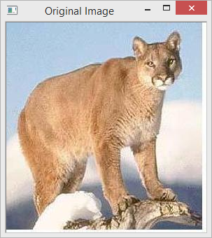
Figure 1: The Original Image

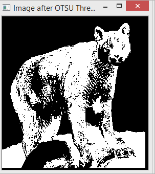
Figure 2: After Applying Otsu's Threshold

After applying Otsu threshold it produces a set of small and large blobs. In order to remove small blobs morphological open is used.

Morphology - Opening

Morphological opening is an application of some primary operators in image processing namely erosion and dilation. The effect of an opening is more like erosion as it removes some of the bright pixels from the edges of regions and some small isolated foreground (bright) pixels. The difference between the basic erosion and opening is that the morphological opening is less destructive than the erosion operation. The reason is that the opening operation is defined as an erosion followed by a dilation using the same structuring element (kernel) for both operations. To read more about morphological opening, see this article. Those who are not familiar with basic image processing operations please read this article so you can get an idea of erosion and dilation.

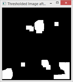
Figure 3: After Applying Morphology-Opening to the Otsu-Thresholded Image

Sometimes some regions are more meaningful if it is partitioned to several subregions. In the case of splitting the regions that has been formed with several subregions connected through a small line or a bunch of pixels, the distance transformation can be used.

Distance Transformation

Distance transformation, distance map or distance field is the process of representing the foreground of an binary image with the distance from the nearest obstacle or background pixel. This process fades-out the the edges and small islands or foregrounds while preserving the region centers.

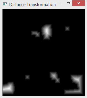
Figure 4: Image After Distance Transformation

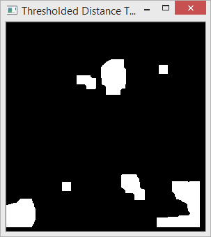
Figure 5: Image After Applying the Threshold to Distance Transformed Image: If there are any loosely connected sub-regions, this step will detach them.

Watershed algorithm can be executed using the foreground patches as the seeds for the algorithm.

Watershed Segmentation Algorithm

Watershed segmentation is a nature inspired algorithm which mimics a phenomena of water flowing through topographic relief. In watershed segmentation an image is considered as topographic relief, where the the gradient magnitude is interpreted as elevation information. Watershed algorithm has been improved with marker controlled flooding technique which you can see as an animation in here. In this implementation we select the markers not by hand but extracting brighter blobs in the image. The above mentioned topics has actually explained this process of marker extraction for watershed segmentation.

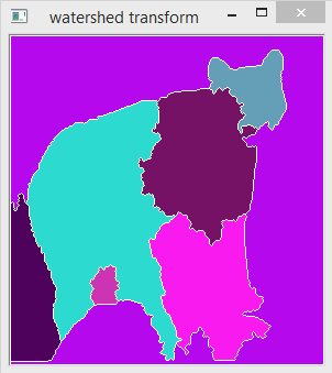
Figure 6: After Applying Watershed Segmentation

The regions with different colours correspond to different segments in the image. In thins image we can see that it has segmented the foreground and background as we can identify the object just by looking at the shapes. But at the same time both the foreground and background segmented to smaller regions which are meaning less when take as an individual piece. This is called as over-segmentation. One method of reducing this over-segmentation is merging the visually similar segments and consider as a single segment.

In computer vision, there are numerous methods available to measure the visual similarity of two regions in an image. The matching technique is actually should selected based on the application. For some applications which has objects with unique textures can use a good texture descriptor. If the set of objects has unique shape then a shape descriptor can be used. In general cases a set of well known descriptors such as SIFT or SURF can be used. But in most cases using a sophisticated description for measure the similarity is not practical due to high computational complexity. Most of the images in general applications (like semantic indexing of images in web) have objects with objects in many kinds of textures, shapes and colors. If we can assume that there is a great probability to have the same spread of colors in different regions in a single object then we can use the color feature to measure the similarity of different segments of an object.

One of the best ways to express the color spread is using a histogram. But histograms of images in RGB color space is not always represent the color spread well enough to all applications. Histograms in HSV (Hue, Saturation and Value) color space is known to perform well in all most all applications that the color information is dominant.

Hue-Saturation Histogram

The hue component of a color corresponds to a one major color where as Saturation and Value corresponds to variations of the colors in Hue component.

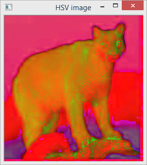
Figure 7: Image in HSV Color Space (Directly applying to imshow() function in openCV)

The image clearly shows that the color spreads in different regions (we extracted using the watershed segmentation) in the same object are similar. Therefore in this implementation a Hue-Saturation histogram is extracted for each region and measure the similarity using a measurement called Bhattacharyya distance. Bhattacharyya distance measures the similarity of two discrete or continuous probability distributions. When the distance is less, the two regions are merged to form a single segment. This merging can be repeated several times if the images has high over-segmentation.

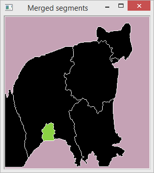
Figure 8: The Segmentation after Merging : Different colours mean different segments. Before merging the segments the black regions appeared in different colours which mean that the object had been over-segmented. But in this image all the segments of the object is merged so the colour is same in all the sub-regions of the object.

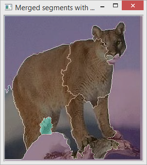
Figure 9: When the Merged Segmentation Mapped to Image

Using the code

The code is developed in VS2008 with c++ and openCV. It has a single source file and all most all the code lines are described with a comment.

The following code line includes the main function where the image is loaded, segment, and show the final result.

int _tmain(int argc, _TCHAR* argv[])
{
    //To store the image file name
    char* filename = new char[50]; 
    //Print image file name to the string
    sprintf(filename,"C:\\img\\6.jpg");     
    //Read the file
    Mat image = imread(filename, CV_LOAD_IMAGE_COLOR);  
    //show original image
    imshow("Original Image",image);
    
    
    //to store the number of segments
    int numOfSegments = 0; 
    //Apply watershed
    Mat segments = watershedSegment(image,numOfSegments);
    //Merge segments in order to reduce over segmentation
    mergeSegments(image,segments, numOfSegments);
    //To display the merged segments
    Mat wshed = createSegmentationDisplay(segments,numOfSegments);
    //To display the merged segments blended with the image
    Mat wshedWithImage = createSegmentationDisplay(segments,numOfSegments,image);

    //Display the merged segments
    imshow("Merged segments",wshed);
    //Display the merged segments blended with the image
    imshow("Merged segments with image",wshedWithImage);

    waitKey(0);
    return 0;
} 

In this code first it loads an image from a local drive. Then display the original image. The segmentation is done using the function watershedSegment. The function produce the segmentation map and the number of segments via numOfSegments.

Then it calls the function mergeSegments to reduce the over-segmentation using histogram matching technique. Once this function call it will merge the regions with similar histograms. Based on the application you may call this function multiple times so the number of segments will be further reduced. The value of the variable numOfSegments will be adjusted according to the actual number of segments as you updated it by calling the function.

The function createSegmentDisplay creates a displayable image with assigning different colors to different segments. If we pass the original image to the function it will blend the segment color code with the original image, so the segmentation will be clearly visible.

These are the steps in brief, of this implementation. The next section will explains the code within the three functions namely watershedSegment, mergeSegments and createSegmentationDisplay.

The watershed algorithm needs a set of markers. These markers are obtained by a set of image processing steps. First the image is converted to grayscale and apply Otsu threshold. The following code does these two steps.

//To store the gray version of the image
Mat gray;
//To store the thresholded image
Mat ret;
//convert the image to grayscale
cvtColor(image,gray,CV_BGR2GRAY);
imshow("Gray Image",gray);
//threshold the image
threshold(gray,ret,0,255,CV_THRESH_BINARY_INV+CV_THRESH_OTSU);
imshow("Image after OTSU Thresholding",ret); 

Then execute morphology-opening with the thresholded image using the following code lines.

//Execute morphological-open
morphologyEx(ret,ret,MORPH_OPEN,Mat::ones(9,9,CV_8SC1),Point(4,4),2);
imshow("Thresholded Image after Morphological open",ret); 

Distance transformation is applied in order to detach any attached sub-regions and threshold the resultant image using the following code lines (the normalization is done for the purpose of displaying the transformed image).

//get the distance transformation 
Mat distTransformed(ret.rows,ret.cols,CV_32FC1);
distanceTransform(ret,distTransformed,CV_DIST_L2,3);
//normalize the transformed image in order to display
normalize(distTransformed, distTransformed, 0.0, 1, NORM_MINMAX);
imshow("Distance Transformation",distTransformed);
//threshold the transformed image to obtain markers for watershed
threshold(distTransformed,distTransformed,0.1,1,CV_THRESH_BINARY);
//Renormalize to 0-255 to further calculations
normalize(distTransformed, distTransformed, 0.0, 255.0, NORM_MINMAX);
distTransformed.convertTo(distTransformed,CV_8UC1);
imshow("Thresholded Distance Transformation",distTransformed); 

After executing these lines we get a set of white markers in an black image. The we need to find the contours of this markers in order to feed the watershed algorithm. This step is done using the following lines of codes.

//calculate the contours of markers
int i, j, compCount = 0;
vector<vector<Point> > contours;
vector<Vec4i> hierarchy;
findContours(distTransformed, contours, hierarchy, CV_RETR_CCOMP, CV_CHAIN_APPROX_SIMPLE);

if( contours.empty() )
    return Mat();
    Mat markers(distTransformed.size(), CV_32S);
    markers = Scalar::all(0);
    int idx = 0;
    //draw contours 
    for( ; idx >= 0; idx = hierarchy[idx][0], compCount++ )
        drawContours(markers, contours, idx, Scalar::all(compCount+1), -1, 8, hierarchy, INT_MAX); 

Finally we can apply the watershed algorithm to the image with the markers as shown in the following lines of code.

//apply watershed with the markers as seeds
    watershed( image, markers ); 

In the mergeSegments function first, a set vector of samples ins created for each segments in the image in order to calculate the histograms. The allocation and pixel collections to the samples are done using the following lines of code.

//To collect pixels from each segment of the image
vector<Mat> samples;
//In case of multiple merging iterations, the numOfSegments should be updated
int newNumOfSegments = numOfSegments;

//Initialize the segment samples
for(int i=0;i<=numOfSegments;i++)
{
    Mat sampleImage;
    samples.push_back(sampleImage);
}

//collect pixels from each segments
for(int i = 0; i < segments.rows; i++ )
{
    for(int j = 0; j < segments.cols; j++ )
    {
        //check what segment the image pixel belongs to
        int index = segments.at<int>(i,j);
        if(index >= 0 && index<numOfSegments)
        {
            samples[index].push_back(image(Rect(j,i,1,1)));    
        }
    }
}  

The variable index holds the segment index of the current pixel at (j,i). Based on the index it populates the samples. After that these samples are used to create HS-histogram. The following lines of code calculate the HS-Histograms for each sample. You can change the code to generate histograms in any dimension as explained in the inline comments.

//create histograms
vector<MatND> hist_bases;
Mat hsv_base;
/// Using 35 bins for hue component 
int h_bins = 35;
/// Using 30 bins for saturation component
int s_bins = 30;
int histSize[] = { h_bins,s_bins };

// hue varies from 0 to 256, saturation from 0 to 180
float h_ranges[] = { 0, 256 };    
float s_ranges[] = { 0, 180 };

const float* ranges[] = { h_ranges, s_ranges };

// Use the 0-th and 1-st channels
int channels[] = { 0,1 };

// To store the histograms
MatND hist_base;
for(int c=1;c<numOfSegments;c++)
{
    if(samples[c].dims>0){
        //convert the sample to HSV
        cvtColor( samples[c], hsv_base, CV_BGR2HSV );
        //calculate the histogram
        calcHist( &hsv_base, 1, channels, Mat(), hist_base,2, histSize, ranges, true, false );
        //normalize the histogram
        normalize( hist_base, hist_base, 0, 1, NORM_MINMAX, -1, Mat() );
        //append to the collection 
        hist_bases.push_back(hist_base);
    }else
    {
        hist_bases.push_back(MatND());
    }
    
    hist_base.release();
} 

Finally the similarity is matched and merge the segments with similar histograms using the following code.

//calculate the similarity of the histograms of each pair of segments
for(int c=0;c<hist_bases.size();c++)
{
    for(int q=c+1;q<hist_bases.size();q++)
    {
        //if the segment is not merged alreay
        if(!mearged[q])
        {
            if(hist_bases[c].dims>0 && hist_bases[q].dims>0)
            {
                //calculate the histogram similarity
                similarity = compareHist(hist_bases[c],hist_bases[q],CV_COMP_BHATTACHARYYA);
                //if similay
                if(similarity>0.8)
                {
                    mearged[q]=true;
                    if(q!=c)
                    {
                        //reduce number of segments
                        newNumOfSegments--;
                        for(int i = 0; i < segments.rows; i++ )
                        {
                            for(int j = 0; j < segments.cols; j++ )
                            {
                                int index = segments.at<int>(i,j);
                                //merge the segment q with c
                                if(index==q){
                                    segments.at<int>(i,j) = c;
                                }
                            }
                        }
                    }
                }
            }
        }
    }
}  

Creation of displayable image out of the segment mask and image is done using the following code lines (When the original image is not available it shows only the colored masks of each segments)

Mat createSegmentationDisplay(Mat & segments,int numOfSegments,Mat & image)
{
    //create a new image
    Mat wshed(segments.size(), CV_8UC3);
    
    //Create color tab for coloring the segments
    vector<Vec3b> colorTab;
    for(int i = 0; i < numOfSegments; i++ )
    {
        int b = theRNG().uniform(0, 255);
        int g = theRNG().uniform(0, 255);
        int r = theRNG().uniform(0, 255);

        colorTab.push_back(Vec3b((uchar)b, (uchar)g, (uchar)r));
    }
    
    //assign different color to different segments
    for(int i = 0; i < segments.rows; i++ )
    {
        for(int j = 0; j < segments.cols; j++ )
        {
            int index = segments.at<int>(i,j);
            if( index == -1 )    
                wshed.at<Vec3b>(i,j) = Vec3b(255,255,255);
            else if( index <= 0 || index > numOfSegments )
                wshed.at<Vec3b>(i,j) = Vec3b(0,0,0);
            else
                wshed.at<Vec3b>(i,j) = colorTab[index - 1]; 
        }
    }

    //If the original image available then merge with the colors of segments
    if(image.dims>0)
        wshed = wshed*0.5+image*0.5;

    return wshed;
} 

If the original image is available then it blends the colored masks with the regions in the original image.

Linux Build Instructions

The original code has been modified to compile in Linux environment, by SoothingMist-Peter, a codeproject member. I am really thankful to him for sharing his achievement with us. The followings are the build instructions shared by him.

1. First download the zip file that contains the source for Linux built.

2. Set environment variables using the terminal as follow.

setenv LD_LIBRARY_PATH $PET_HOME/.unsupported/opencv-2.4.8/lib:$LD_LIBRARY_PATH   

Note: You should replace the part of line $PET_HOME/.unsupported/opencv-2.4.8/lib with the path where you installed openCV lib folder.

3. Unload any conflicting pre-loaded modules and load the gcc module as follow. Make necessary changes to support this script to the module versions installed in your computer.

module unload compiler/pgi/13.3
module unload mpi/pgi/openmpi/1.6.3
module load compiler/gcc/4.4
module list

4. Compile the file AutoSeedWatershed.cpp from its current directory using the following script.

g++ AutoSeedWatershed.cpp -o AutoSeedWatershed `pkg-config $PET_HOME/.unsupported/opencv-2.4.8/lib/pkgconfig/opencv.pc --cflags --libs`  

5. Now you can run the program as following.

./AutoSeedWatershed   

Points of Interest

I tested this code for several images which are taken from a standard dataset for image classification researches. But it does not mean that this code should works for images in all domains. Images in different domains may require a fine tuning or a modification in some parts of the code. The most important parts are finding markers for the watershed algorithm and calculating the similarity of different segments in order to reduce the over-segmentation. You can apply different approach as there are lot of ways to do the same. Try this code and you are always welcome to ask questions, make suggestions and any comment regarding the code or the article.