This post will show you some updates in TensorFlow 2.0 and how to create a linear regression model from scratch.
Introduction
On September 30, 2019, Google announced that the final release of TensorFlow 2.0 (TF 2.0) is now available. From TensorFlow Guide, there are major changes in TF 2.0:
- Removing redundant APIs such as
tf.app, tf.flags, tf.logging. - Executing eagerly like Python (Eager execution)
- Keeping track of your variables and if you lose track of a
tf.Variable, TF 2.0 gets garbage collected. - Using
tf.function.
You can discover more about new changes in TF 2.0 at TensorFlow Guide. In this post, I will represent some changes in TF 2.0 by creating linear regression models from scratch.
Background
In one of my older articles, I introduced the linear regression algorithm and how to create a simple linear regression model using TensorFlow 1.X. In this post, I will update that model (with 2 weights) to TF 2.0 and I also create a model with more weights (of course, more than 2).
Using the Code
Simple Linear Regression Model (With Two Weights)
In TensorFlow 1.X, I created a model and implemented it with the following lines of code:
...
w0 = tf.Variable(0.0, name="w0")
w1 = tf.Variable(0.0, name="w1")
...
train_op = tf.train.GradientDescentOptimizer(learning_rate).minimize(costF)
sess = tf.Session()
init = tf.global_variables_initializer()
sess.run(init)
for epoch in range(training_epochs):
for (x, y) in zip(x_train, y_train):
sess.run(train_op, feed_dict={X: x, Y: y})
w_val_0 = sess.run(w0)
w_val_1 = sess.run(w1)
As code above, in TF 1.X, we must:
- declare variables (
tf.Varialble) and initialize these variables (tf.global_variables_initializer) before using them. - train our model using
tf.train.GradientDescentOptimizer. - set up (
tf.Session) and run the session to execute operations in the graph.
In TF 2.0, we will:
- declare variables (
tf.Variable) but don't need to use tf.global_variables_initializer, that means, TensorFlow 2.0 doesn’t make it mandatory to initialize variables. - train our model using tf.GradientTape and we will use assign_sub for weight variables.
- not require the session execution.
From the main points above, we will re-create our linear regression model with two weights as follows:
import tensorflow as tf
import numpy as np
import matplotlib.pyplot as plt
learning_rate = 0.01
training_epochs = 100
x_train = np.linspace(0, 10, 100)
y_train = x_train + np.random.normal(0,1,100)
w0 = tf.Variable(0.)
w1 = tf.Variable(0.)
def h(x):
y = w1*x + w0
return y
def squared_error(y_pred, y_true):
return tf.reduce_mean(tf.square(y_pred - y_true))
for epoch in range(training_epochs):
with tf.GradientTape() as tape:
y_predicted = h(x_train)
costF = squared_error(y_predicted, y_train)
gradients = tape.gradient(costF, [w1,w0])
w1.assign_sub(gradients[0]*learning_rate)
w0.assign_sub(gradients[1]*learning_rate)
plt.scatter(x_train, y_train)
plt.plot(x_train, h(x_train), 'r')
plt.show()
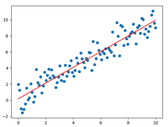
If we run this script, the result can look like this:

Polynomial Model
When data points appear to form smooth curves rather than straight lines, we need to change our regression model from a straight line to something else. One such approach is to use a polynomial model. A polynomial is a generalization of a linear function. The following lines of code will create a polynomial model:
import tensorflow as tf
import numpy as np
import matplotlib.pyplot as plt
learning_rate = 0.05
training_epochs = 100
x_train = np.linspace(-1, 1, 101)
num_coeffs = 6
trY_coeffs = [1, 2, 3, 4, 5, 6]
y_train = 0
for i in range(num_coeffs):
y_train += trY_coeffs[i] * np.power(x_train, i)
y_train += np.random.randn(*x_train.shape) * 1.5
w = tf.Variable([0.] * num_coeffs, name="parameters")
def h(x):
y = 0
for i in range(num_coeffs):
y += w[i]*pow(x,i)
return y
def squared_error(y_pred, y_true):
return tf.reduce_mean(tf.square(y_pred - y_true))
for epoch in range(training_epochs):
with tf.GradientTape() as tape:
y_predicted = h(x_train)
costF = squared_error(y_predicted, y_train)
gradients = tape.gradient(costF, w)
w.assign_sub(gradients*learning_rate)
plt.scatter(x_train, y_train)
plt.plot(x_train, h(x_train), 'r')
plt.show()
If we run this script, the result can look like this:

Of course, we need to improve this model but I don't do that in this post.
Points of Interest
TensorFlow is a great platform for deep learning and machine learning and TF 2.0 focuses on simplicity and ease of use. In this post, I introduced some new changes in TF 2.0 by building simple linear regression models from scratch (don't use APIs such as Keras) and I hope you feel excited about it.
History
- 25th March, 2020: Initial version
